


 本文深入探讨了使用Python进行机器学习的实践案例,包括肿瘤预测、新闻分类、MNIST手写数字识别等,涵盖多种算法如逻辑回归、支持向量机、朴素贝叶斯等。
书籍《Python机器学习及实践》阅读笔记
分类问题
一、使用两个属性的肿瘤预测-LR
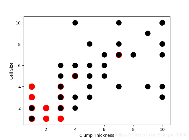
使用数据集中的两个属性进行肿瘤预测,计算准确率并绘图
import pandas as pd
import matplotlib.pyplot as plt
import numpy as np
from sklearn.linear_model import LogisticRegression
from sklearn.svm import SVR
#---------read data
df_train = pd.read_csv('./Datasets/Breast-cancer/breast-cancer-train.csv')
df_test = pd.read_csv('./Datasets/Breast-cancer/breast-cancer-test.csv')
df_test_negative = df_test.loc[df_test['Type'] == 0][['Clump Thickness','Cell Size']]
df_test_positive = df_test.loc[df_test['Type'] == 1][['Clump Thickness','Cell Size']]
#--------image 1
plt.scatter(df_test_negative['Clump Thickness'], df_test_negative['Cell Size'], marker='o', s=200, c = 'red')
plt.scatter(df_test_positive['Clump Thickness'], df_test_positive['Cell Size'], marker='o', s=150, c = 'black')
plt.xlabel('Clump Thickness')
plt.ylabel('Cell Size')
plt.show()
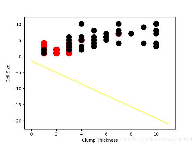
#---------image 2
intercept = np.random.random([1])
coef = np.random.random([2])
lx = np.arange(0,12)
ly = (-intercept-lx*coef[0])/coef[1]
plt.plot(lx,ly,c='yellow')
plt.scatter(df_test_negative['Clump Thickness'], df_test_negative['Cell Size'], marker='o', s=200, c = 'red')
plt.scatter(df_test_positive['Clump Thickness'], df_test_positive['Cell Size'], marker='o', s=150, c = 'black')
plt.xlabel('Clump Thickness')
plt.ylabel('Cell Size')
plt.show()
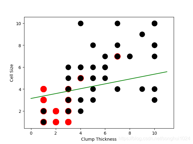
#--------learn with 10 samples
lr = LogisticRegression()
lr.fit(df_train[['Clump Thickness', 'Cell Size']][:10],df_train['Type'][:10])
acc = lr.score(df_test[['Clump Thickness','Cell Size']],df_test['Type'])
print("Testing accuracy (10 training samples): {sc}".format(sc=acc))
#--------draw learn result
intercept = lr.intercept_
coef = lr.coef_[0,:]
ly = (-intercept-lx*coef[0])/coef[1]
plt.plot(lx,ly,c='green')
plt.scatter(df_test_negative['Clump Thickness'], df_test_negative['Cell Size'], marker='o', s=200, c = 'red')
plt.scatter(df_test_positive['Clump Thickness'], df_test_positive['Cell Size'], marker='o', s=150, c = 'black')
plt.xlabel('Clump Thickness')
plt.ylabel('Cell Size')
plt.show()
#-----------learn with all training data
lr = LogisticRegression()
lr.fit(df_train[['Clump Thickness', 'Cell Size']],df_train['Type'])
acc = lr.score(df_test[['Clump Thickness','Cell Size']],df_test['Type'])
print("Testing accuracy (all training samples): {sc}".format(sc=acc))
#-----------draw learn result
plt.plot(lx,ly,c='green')
plt.scatter(df_test_negative['Clump Thickness'], df_test_negative['Cell Size'], marker='o', s=200, c = 'red')
plt.scatter(df_test_positive['Clump Thickness'], df_test_positive['Cell Size'], marker='o', s=150, c = 'black')
plt.xlabel('Clump Thickness')
plt.ylabel('Cell Size')
plt.show()
lr = SVR()
lr.fit(df_train[['Clump Thickness', 'Cell Size']],df_train['Type'])
acc = lr.score(df_test[['Clump Thickness','Cell Size']],df_test['Type'])
print("Testing accuracy (all training samples with SVM): {sc}".format(sc=acc))
----------------------------
output:
Testing accuracy (10 training samples): 0.8685714285714285
Testing accuracy (all training samples): 0.9371428571428572
Testing accuracy (all training samples with SVM): 0.7771531127280293

二、使用多个属性的肿瘤预测-LR&SGD
LR采用精确解析方式,计算时间长但模型性能略高,SGD采用随机梯度下降方式,计算时间短但是模型性能略低;对于10万级以上数据,考虑到时间的耗用,随机梯度下降更好一些。
import pandas as pd
import numpy as np
from sklearn.model_selection import train_test_split
from sklearn.preprocessing import StandardScaler
from sklearn.linear_model import LogisticRegression
from sklearn.linear_model import SGDClassifier
from sklearn.metrics import classification_report

column_names = ['Sample code number','Clump Thickness', 'Uniformity of Cell Size',
                'Uniformity of Cell Shape', 'Marginal Adhesion', 'Single Epithelial Cell Size',
                'Bare Nuclei','Bland Chromatin', 'Normal Nucleoli', 'Mitoses', 'Class']
data = pd.read_csv('./Datasets/Breast-Cancer/breast-cancer-wisconsin.data',names=column_names)
data = data.replace(to_replace='?',value=np.nan)
data = data.dropna(how='any')
#print(data)
#print(data.shape)

X_train, X_test, y_train, y_test = \
    train_test_split(data[column_names[1:10]],data[column_names[10]],test_size=.25,random_state=33)
#print(y_train.value_counts())
#print(y_test.value_counts())
ss=StandardScaler()
X_train = ss.fit_transform(X_train)
X_test = ss.transform(X_test)

lr = LogisticRegression()
sgdc = SGDClassifier()
lr.fit(X_train,y_train)
lr_y_predict=lr.predict(X_test)
sgdc.fit(X_train,y_train)
sgdc_y_predict = sgdc.predict(X_test)

print("Accuracy of LR Classifier: {sc}".format(sc=lr.score(X_test, y_test)))
print(classification_report(y_test,lr_y_predict,target_names=['Benign','Malignant']))

print("Accuracy of SGD Classifier: {sc}".format(sc=sgdc.score(X_test, y_test)))
print(classification_report(y_test,sgdc_y_predict,target_names=['Benign','Malignant']))
-----------------
output:
Accuracy of LR Classifier: 0.9883040935672515

             precision    recall  f1-score   support
     Benign       0.99      0.99      0.99       100
  Malignant       0.99      0.99      0.99        71

avg / total       0.99      0.99      0.99       171
-----------------------------------------------------
Accuracy of SGD Classifier: 0.9649122807017544
             precision    recall  f1-score   support

     Benign       0.98      0.96      0.97       100
  Malignant       0.95      0.97      0.96        71

avg / total       0.97      0.96      0.96       171
三、mnist-SVM,LR,SGD
from sklearn.datasets import load_digits
from sklearn.model_selection import train_test_split
from sklearn.preprocessing import StandardScaler
from sklearn.svm import LinearSVC
from sklearn.metrics import classification_report
from sklearn.linear_model import LogisticRegression
from sklearn.linear_model import SGDClassifier

digits = load_digits()
print(digits.data.shape)
print(type(digits.data))

X_train, X_test, y_train, y_test = train_test_split(digits.data, digits.target,test_size=.25, random_state=33)
print(y_train.shape)
print(y_test.shape)

ss = StandardScaler()
X_train = ss.fit_transform(X_train)
X_test = ss.transform(X_test)

lsvc = LinearSVC()
lsvc.fit(X_train,y_train)
y_predict = lsvc.predict(X_test)

print("The Accuracy of Linear SVC is: {sc}".format(sc = lsvc.score(X_test,y_test)))
print(classification_report(y_test, y_predict, target_names=digits.target_names.astype(str)))

lr = LogisticRegression()
lr.fit(X_train,y_train)
lr_y_predict = lr.predict(X_test)

print("The Accuracy of Linear Regression is: {sc}".format(sc = lr.score(X_test,y_test)))
print(classification_report(y_test, lr_y_predict, target_names=digits.target_names.astype(str)))

sgdc = SGDClassifier()
sgdc.fit(X_train,y_train)
sgdc_y_predict = sgdc.predict(X_test)

print("Accuracy of SGD Classifier: {sc}".format(sc=sgdc.score(X_test, y_test)))
print(classification_report(y_test,sgdc_y_predict,target_names=digits.target_names.astype(str)))
---------------------------
output:
(1797, 64)
<class 'numpy.ndarray'>
(1347,)
(450,)
The Accuracy of Linear SVC is: 0.9533333333333334
             precision    recall  f1-score   support

          0       0.92      1.00      0.96        35
          1       0.96      0.98      0.97        54
          2       0.98      1.00      0.99        44
          3       0.93      0.93      0.93        46
          4       0.97      1.00      0.99        35
          5       0.94      0.94      0.94        48
          6       0.96      0.98      0.97        51
          7       0.92      1.00      0.96        35
          8       0.98      0.84      0.91        58
          9       0.95      0.91      0.93        44

avg / total       0.95      0.95      0.95       450

The Accuracy of Linear Regression is: 0.96
             precision    recall  f1-score   support

          0       0.95      1.00      0.97        35
          1       0.93      0.98      0.95        54
          2       1.00      1.00      1.00        44
          3       0.96      0.96      0.96        46
          4       1.00      0.94      0.97        35
          5       0.98      0.94      0.96        48
          6       0.96      0.98      0.97        51
          7       0.95      1.00      0.97        35
          8       0.98      0.88      0.93        58
          9       0.91      0.95      0.93        44

avg / total       0.96      0.96      0.96       450


Accuracy of SGD Classifier: 0.9555555555555556
             precision    recall  f1-score   support

          0       1.00      1.00      1.00        35
          1       0.95      0.98      0.96        54
          2       1.00      0.95      0.98        44
          3       0.95      0.91      0.93        46
          4       1.00      0.94      0.97        35
          5       0.94      0.94      0.94        48
          6       0.96      0.98      0.97        51
          7       0.97      1.00      0.99        35
          8       0.92      0.93      0.92        58
          9       0.91      0.93      0.92        44

avg / total       0.96      0.96      0.96       450
四、NewsClassification-NB
朴素贝叶斯假设各个维度上的特征被分类的条件概率之间是相互独立的。这使模型预测所需要估计的参数规模从从幂指数量级向线性量级减少,极大的节约了内存消耗和计算时间。但是,模型无法将各个特征之间的联系考虑在内,使模型在数据集关联性较强的分类任务上性能表现不佳。
from sklearn.datasets import fetch_20newsgroups
from sklearn.model_selection import train_test_split
from sklearn.feature_extraction.text import CountVectorizer
from sklearn.naive_bayes import  MultinomialNB
from sklearn.metrics import classification_report

news = fetch_20newsgroups(subset='all')
print(len(news.data))
print(news.data[0])

X_train, X_test, y_train, y_test = train_test_split(news.data, news.target, test_size=.25, random_state=33)

vec = CountVectorizer()
X_train = vec.fit_transform(X_train)
X_test = vec.transform(X_test)

mnb = MultinomialNB()
mnb.fit(X_train, y_train)
mnb_y_predict = mnb.predict(X_test)

print("The accuracy of NB Classifier is: {sc}".format(sc=mnb.score(X_test,y_test)))
print(classification_report(y_test, mnb_y_predict,target_names=news.target_names))
--------------------------
output:
18846
The accuracy of NB Classifier is: 0.8397707979626485
                          precision    recall  f1-score   support

             alt.atheism       0.86      0.86      0.86       201
           comp.graphics       0.59      0.86      0.70       250
 comp.os.ms-windows.misc       0.89      0.10      0.17       248
comp.sys.ibm.pc.hardware       0.60      0.88      0.72       240
   comp.sys.mac.hardware       0.93      0.78      0.85       242
          comp.windows.x       0.82      0.84      0.83       263
            misc.forsale       0.91      0.70      0.79       257
               rec.autos       0.89      0.89      0.89       238
         rec.motorcycles       0.98      0.92      0.95       276
      rec.sport.baseball       0.98      0.91      0.95       251
        rec.sport.hockey       0.93      0.99      0.96       233
               sci.crypt       0.86      0.98      0.91       238
         sci.electronics       0.85      0.88      0.86       249
                 sci.med       0.92      0.94      0.93       245
               sci.space       0.89      0.96      0.92       221
  soc.religion.christian       0.78      0.96      0.86       232
      talk.politics.guns       0.88      0.96      0.92       251
   talk.politics.mideast       0.90      0.98      0.94       231
      talk.politics.misc       0.79      0.89      0.84       188
      talk.religion.misc       0.93      0.44      0.60       158

             avg / total       0.86      0.84      0.82      4712
五、K近邻-iris
只是根据测试样本在训练数据的分布直接做出决策。因此,K近邻属于无参模型中非常简单的一种。因为该模型每处理一个测试样本,都需要对多有预先加载在内存的训练样本进行遍历、逐一计算相似度、排序,并且选取K个最近邻训练样本的标记,进而做出分类决策,所以,算法具有非常高的计算复杂度和内存消耗。
from sklearn.datasets import load_iris
from sklearn.model_selection import train_test_split
from sklearn.preprocessing import StandardScaler
from sklearn.neighbors import KNeighborsClassifier
from sklearn.metrics import classification_report

iris = load_iris()
print(iris.DESCR)
X_train, X_test, y_train, y_test = train_test_split(iris.data, iris.target, test_size=.25, random_state=33)
ss = StandardScaler()
X_train = ss.fit_transform(X_train)
X_test = ss.transform(X_test)
knc = KNeighborsClassifier()
knc.fit(X_train, y_train)
y_predict = knc.predict(X_test)
print("The accuracy of K-Nearest Neighbor Classifier is: {sc}".format(sc=knc.score(X_test, y_test)))
print(classification_report(y_test, y_predict, target_names=iris.target_names))

----------------
output:
The accuracy of K-Nearest Neighbor Classifier is: 0.8947368421052632
             precision    recall  f1-score   support

     setosa       1.00      1.00      1.00         8
 versicolor       0.73      1.00      0.85        11
  virginica       1.00      0.79      0.88        19

avg / total       0.92      0.89      0.90        38
六、决策树--titantic生还预测
可以用来描述非线性关系,如预测患流感的死亡率、信用卡申请的审核。
相比其他学习模型,决策树在模型描述上有着巨大的优势。推断逻辑非常直观,具有清晰的可解释性,也方便模型可视化。
import pandas as pd
from sklearn.model_selection import train_test_split
from sklearn.feature_extraction import DictVectorizer
from sklearn.tree import DecisionTreeClassifier
from sklearn.metrics import classification_report

titanic = pd.read_csv("http://biostat.mc.vanderbilt.edu/wiki/pub/Main/DataSets/titanic.txt")
#观察前几行数据,可以发现,数据种类各异,数值型,类别型,甚至还有缺失数据
print(titanic.head())
print(titanic.info())
#特征选择:根据我们对这场事故的了解,sex,age,pclass这些特征都很有可能是决定是否幸免的关键因素
X = titanic[['pclass', 'age', 'sex']]
y = titanic['survived']
#对当前选择的特征进行探查
print(X.info())
#(1)age数据列,只有633个,需要补完
#(2)sex与pclass两个数据列都是类别型的,需要转化为数值特征,用0/1表示
#用平均数或者中位数 都是对模型偏离造成最小影响的策略
X['age'].fillna(X['age'].mean(), inplace=True)
print(X.info())

X_train, X_test, y_train, y_test = train_test_split(X, y, test_size=.25, random_state=33)
vec = DictVectorizer(sparse=False)
#转换特征后,类别特征被单独剥离出来,独立成一列特征,数值型则保持不变
X_train = vec.fit_transform(X_train.to_dict(orient='record'))
print(vec.feature_names_)
X_test = vec.transform(X_test.to_dict(orient='record'))
dtc = DecisionTreeClassifier()
dtc.fit(X_train, y_train)
y_predict = dtc.predict(X_test)
print("The accuracy of DecisionTreeClassifier is: {sc}".format(sc=dtc.score(X_test, y_test)))
print(classification_report(y_test,y_predict,target_names=['died','survived']))

----------
output:
['age', 'pclass=1st', 'pclass=2nd', 'pclass=3rd', 'sex=female', 'sex=male']
The accuracy of DecisionTreeClassifier is: 0.7811550151975684
             precision    recall  f1-score   support

       died       0.78      0.91      0.84       202
   survived       0.80      0.58      0.67       127

avg / total       0.78      0.78      0.77       329
七、集成模型
集成分类模型综合考量多个分类器的预测结果,从而做出决策。方式大体上分为两种:
(1)利用相同的训练数据同时搭建多个独立的分类模型,然后通过投票的方式,以少数服从多数的原则做出最终的决策。具有代表性的模型为随机森林分类器(Random Forest Classfier)。
(2)按照一定次序搭建多个分类模型。每个后续加入的模型要对现有集成模型的综合性能有所贡献,进而不断提升更新过后的集成模型的性能,并最终期望借助整合多个分类能力较弱的分类器,搭建具有更强分类能力的模型。具有代表性的模型是梯度提升决策树(Gradient Tree Boosting)。与随机森林分类器不同,每一棵决策树在生成过程中都会尽可能降低整体集成模型在训练集上的拟合误差。
code:利用单一决策树、随机森林分类以及梯度上升决策树,3种模型各自默认配置进行初始化,对比性能。
在相同训练集和测试数据条件下,仅仅使用模型默认配置,梯度上升决策树具有最佳的预测性能,其次是随机森林分类器,最后是单一决策树。一般而言,工业界为了追求强劲的预测性能,经常使用随机森林分类模型作为基线系统。集成模型虽然在训练过程中要耗费更多时间,但是得到的综合模型往往具有更高的表现性能和更好的稳定性。
import pandas as pd
from sklearn.model_selection import train_test_split
from sklearn.feature_extraction import DictVectorizer
from sklearn.tree import DecisionTreeClassifier
from sklearn.metrics import classification_report
from sklearn.ensemble import RandomForestClassifier
from sklearn.ensemble import GradientBoostingClassifier

titanic = pd.read_csv("http://biostat.mc.vanderbilt.edu/wiki/pub/Main/DataSets/titanic.txt")
X = titanic[['pclass', 'age', 'sex']]
y = titanic['survived']
X['age'].fillna(X['age'].mean(), inplace=True)
X_train, X_test, y_train, y_test = train_test_split(X, y, test_size=.2, random_state=11)
vec = DictVectorizer(sparse=False)
#转换特征后,类别特征被单独剥离出来,独立成一列特征,数值型则保持不变
X_train = vec.fit_transform(X_train.to_dict(orient='record'))
X_test = vec.transform(X_test.to_dict(orient='record'))

#使用单一决策树进行模型训练及预测分析
dtc = DecisionTreeClassifier()
dtc.fit(X_train, y_train)
dtc_y_predict = dtc.predict(X_test)

#使用个随机森林分类器进行集成模型训练以及预测分析
rfc = RandomForestClassifier()
rfc.fit(X_train, y_train)
rfc_y_predict = rfc.predict(X_test)

#使用梯度提升决策树进行集成模型的训练及预测分析
gbc = GradientBoostingClassifier()
gbc.fit(X_train, y_train)
gbc_y_predict = gbc.predict(X_test)


print("The accuracy of DecisionTreeClassifier is: {sc}".format(sc=dtc.score(X_test, y_test)))
print(classification_report(y_test, dtc_y_predict, target_names=['died','survived']))

print("The accuracy of RandomForestClassifier is: {sc}".format(sc=rfc.score(X_test, y_test)))
print(classification_report(y_test, rfc_y_predict, target_names=['died','survived']))

print("The accuracy of GradientBoostingClassifier is: {sc}".format(sc=gbc.score(X_test, y_test)))
print(classification_report(y_test, gbc_y_predict, target_names=['died','survived']))
------------
output:
The accuracy of DecisionTreeClassifier is: 0.7718631178707225
             precision    recall  f1-score   support

       died       0.76      0.92      0.83       159
   survived       0.81      0.55      0.66       104

avg / total       0.78      0.77      0.76       263

The accuracy of RandomForestClassifier is: 0.7908745247148289
             precision    recall  f1-score   support

       died       0.78      0.91      0.84       159
   survived       0.82      0.61      0.70       104

avg / total       0.79      0.79      0.78       263

The accuracy of GradientBoostingClassifier is: 0.8022813688212928
             precision    recall  f1-score   support

       died       0.77      0.95      0.85       159
   survived       0.88      0.58      0.70       104

avg / total       0.82      0.80      0.79       263


 3019
3019

 被折叠的 条评论
为什么被折叠?
被折叠的 条评论
为什么被折叠?
 到【灌水乐园】发言


