tensorflow-代码-非线性回归

tensorflow之路 六：非线性回归

通过代码能够实现一个：输入层为一个神经元，隐藏层为10个神经元，输出层为一个神经元的神经网络模型。

输入为：-1至1随机初始化的500个点作为x值

代码：

import tensorflow as tf
import numpy as np
import matplotlib.pyplot as plt

#使用numpy生成500样本点
x_data = np.linspace(-1,1,500)[:,np.newaxis]#将数据变为200行一列数据
print(x_data.shape)
noise = np.random.normal(0,0.5,x_data.shape)#创建一个噪声数据
y_data = np.square(x_data) + noise#函数为x的平方+噪声，得到原始数据y值

#定义两个placeholder
x = tf.placeholder(tf.float32,[None,1])#浮点型数据，n行1列
y = tf.placeholder(tf.float32,[None,1])

#定义神经网络中间层，
Weight_L1 = tf.Variable(tf.random_normal([1,10]))#输入层1个神经元，输出层10个神经元
biases_L1 = tf.Variable(tf.zeros([1,10]))#初始偏置值为0
Wx_plus_L1 = tf.matmul(x,Weight_L1)+ biases_L1

#使用激活函数激活
L1 = tf.nn.tanh(Wx_plus_L1)

#定义输出层
Weight_L2 = tf.Variable(tf.random_normal([10,1]))
biases_L2 = tf.Variable(tf.zeros([1,1]))

Wx_plus_L2 = tf.matmul(L1,Weight_L2) + biases_L2

prediction = tf.nn.tanh(Wx_plus_L2)

#二次代价函数
loss = tf.reduce_mean(tf.square(y-prediction))
#使用梯度下降法
train_step = tf.train.GradientDescentOptimizer(0.1).minimize(loss)

with tf.Session() as sess:
    sess.run(tf.global_variables_initializer())
    for _ in range(2000):
        sess.run(train_step,feed_dict={x:x_data,y:y_data})

    #获得预测值
    prediction_value = sess.run(prediction,feed_dict={x:x_data})

    #画图
    plt.figure()
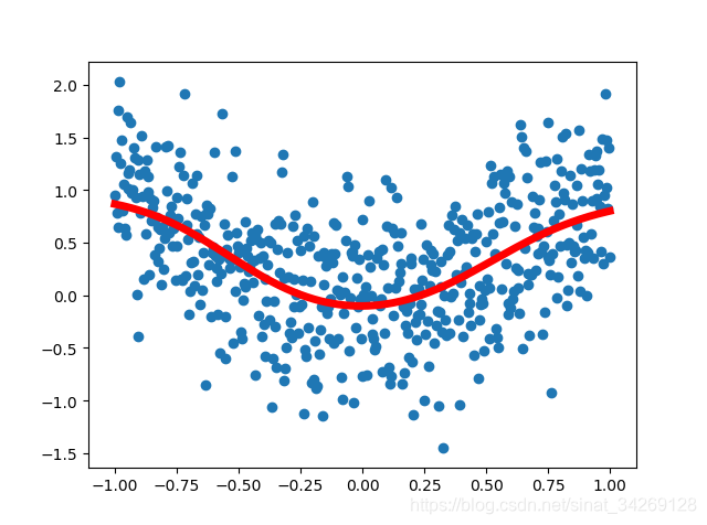
    plt.scatter(x_data,y_data)
    plt.plot(x_data,prediction_value,'r-',lw=5)
    plt.show()

画图显示结果：蓝色点为原始初始化的200个点，红色为预测出的结果