XGBoost实战: 保险赔偿预测_保险赔偿预测—

本文链接：https://blog.youkuaiyun.com/sanjianjixiang/article/details/105887047

本文详细介绍了使用XGBoost进行保险赔偿预测的过程，包括数据查看、特征离散值与连续值分析、目标变量处理、数据预处理、建立基本模型以及通过交叉验证进行模型调参，如改变max_depth、min_child_weight、gamma、subsample和colsample_bytree，并逐步减小学习率和增加树的数量以提升模型性能。

摘要生成于 C知道，由 DeepSeek-R1 满血版支持，前往体验 >

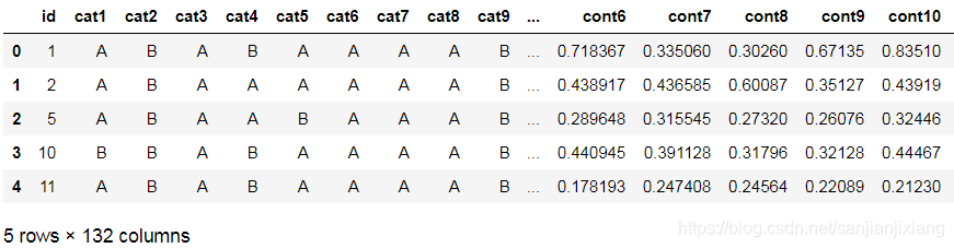
一. 查看数据

import numpy as np
import pandas as pd
import matplotlib.pyplot as plt
import seaborn as sns
%matplotlib inline

train = pd.read_csv(r'F:\51学习\study\数据挖掘案例\Xgboost调参\Xgboost\train.csv')
test = pd.read_csv(r'F:\51学习\study\数据挖掘案例\Xgboost调参\Xgboost\test.csv')
print(train.shape)
print(test.shape)
train.head()

(188318, 132)
(125546, 131)
在这里插入图片描述

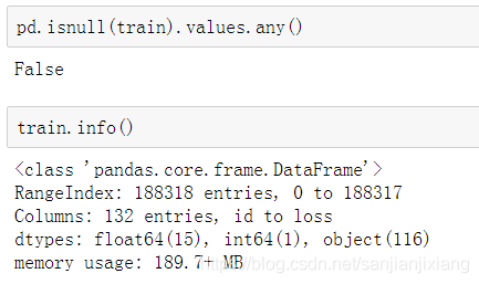
1.1 离散值

cat_features = list(train.select_dtypes(include = 'object').columns)
print('Categorical: {} features.'.format(len(cat_features)))

cont_features = [cont for cont in list(train.select_dtypes(
                include = ['float64', 'int64']).columns) if cont not in ['loss', 'id']]
print('Continuous: {} features.'.format(len(cont_features)))

id_col = list(train.select_dtypes(include = 'int64').columns)
print('A column of int64: {}.'.format(id_col))

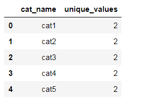
# 类别值中属性的个数
categorical_uniques = []
for cat in cat_features:
    categorical_uniques.append(len(train[cat].unique()))
uniq_values_in_categories = pd.DataFrame.from_dict({
   
   'cat_name':cat_features, 'unique_values':categorical_uniques})
uniq_values_in_categories.head()

Categorical: 116 features.
Continuous: 14 features.
A column of int64: [‘id’].
在这里插入图片描述

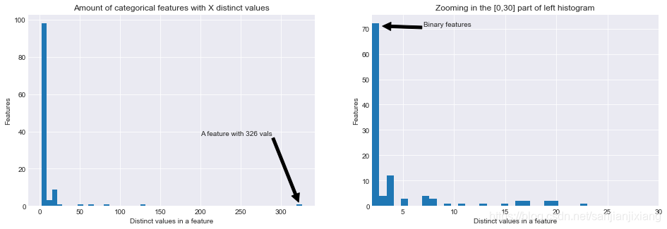
plt.style.use('seaborn-darkgrid')
fig, (ax1, ax2) = plt.subplots(1, 2, figsize = (16, 5))

ax1.hist(uniq_values_in_categories.unique_values, bins = 50)
ax1.set_title('Amount of categorical features with X distinct values')
ax1.set_xlabel('Distinct values in a feature')
ax1.set_ylabel('Features')
ax1.annotate('A feature with 326 vals', xy=(322, 2), xytext=(200, 38), arrowprops=dict(facecolor='black'))

ax2.hist(uniq_values_in_categories[uniq_values_in_categories.unique_values <= 30].unique_values, bins = 30)
ax2.set_xlim(2, 30)
ax2.set_title('Zooming in the [0,30] part of left histogram')
ax2.set_xlabel('Distinct values in a feature')
ax2.set_ylabel('Features')
ax2.annotate('Binary features', xy = (3, 71), xytext = (7, 71), arrowprops = dict(facecolor = 'black'))

在这里插入图片描述

1.2 目标值

plt.figure(figsize = (12, 6))
plt.plot(train['id'], train['loss'])
plt.title('Loss values per id')
plt.xlabel('Id')
plt.ylabel('loss')

在这里插入图片描述
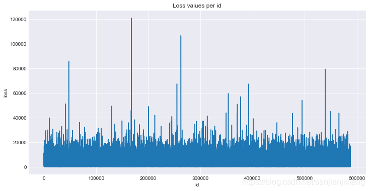
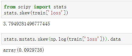
数据时倾斜的, 可使用np.log改善倾斜度:

fig, (ax1, ax2) = plt.subplots(1, 2)
fig.set_size_inches(14, 5)

ax1.hist(train['loss'], bins = 50)
ax1.set_title('Train Loss target histogram')

ax2.hist(np.log(train['loss']), bins = 50, color