BaseMap根据震中距和震中画圆圈

#
# BaseMap example by geophysique.be
# tutorial 09
from mpl_toolkits.basemap import Basemap
import matplotlib.pyplot as plt
 
import numpy as np
 
### PARAMETERS FOR MATPLOTLIB :
import matplotlib as mpl
mpl.rcParams['font.size'] = 10.
mpl.rcParams['font.family'] = 'Comic Sans MS'
mpl.rcParams['axes.labelsize'] = 8.
mpl.rcParams['xtick.labelsize'] = 6.
mpl.rcParams['ytick.labelsize'] = 6.
 
def shoot(lon, lat, azimuth, maxdist=None):
    """Shooter Function
    Original javascript on http://williams.best.vwh.net/gccalc.htm
    Translated to python by Thomas Lecocq
    """
    glat1 = lat * np.pi / 180.
    glon1 = lon * np.pi / 180.
    s = maxdist / 1.852
    faz = azimuth * np.pi / 180.
 
    EPS= 0.00000000005
    if ((np.abs(np.cos(glat1))<EPS) and not (np.abs(np.sin(faz))<EPS)):
        alert("Only N-S courses are meaningful, starting at a pole!")
 
    a=6378.13/1.852
    f=1/298.257223563
    r = 1 - f
    tu = r * np.tan(glat1)
    sf = np.sin(faz)
    cf = np.cos(faz)
    if (cf==0):
        b=0.
    else:
        b=2. * np.arctan2 (tu, cf)
 
    cu = 1. / np.sqrt(1 + tu * tu)
    su = tu * cu
    sa = cu * sf
    c2a = 1 - sa * sa
    x = 1. + np.sqrt(1. + c2a * (1. / (r * r) - 1.))
    x = (x - 2.) / x
    c = 1. - x
    c = (x * x / 4. + 1.) / c
    d = (0.375 * x * x - 1.) * x
    tu = s / (r * a * c)
    y = tu
    c = y + 1
    while (np.abs (y - c) > EPS):
 
        sy = np.sin(y)
        cy = np.cos(y)
        cz = np.cos(b + y)
        e = 2. * cz * cz - 1.
        c = y
        x = e * cy
        y = e + e - 1.
        y = (((sy * sy * 4. - 3.) * y * cz * d / 6. + x) *
              d / 4. - cz) * sy * d + tu
 
    b = cu * cy * cf - su * sy
    c = r * np.sqrt(sa * sa + b * b)
    d = su * cy + cu * sy * cf
    glat2 = (np.arctan2(d, c) + np.pi) % (2*np.pi) - np.pi
    c = cu * cy - su * sy * cf
    x = np.arctan2(sy * sf, c)
    c = ((-3. * c2a + 4.) * f + 4.) * c2a * f / 16.
    d = ((e * cy * c + cz) * sy * c + y) * sa
    glon2 = ((glon1 + x - (1. - c) * d * f + np.pi) % (2*np.pi)) - np.pi    
 
    baz = (np.arctan2(sa, b) + np.pi) % (2 * np.pi)
 
    glon2 *= 180./np.pi
    glat2 *= 180./np.pi
    baz *= 180./np.pi
 
    return (glon2, glat2, baz)
 
def equi(m, centerlon, centerlat, radius, *args, **kwargs):
    glon1 = centerlon
    glat1 = centerlat
    X = []
    Y = []
    for azimuth in range(0, 360):
        glon2, glat2, baz = shoot(glon1, glat1, azimuth, radius)
        X.append(glon2)
        Y.append(glat2)
    X.append(X[0])
    Y.append(Y[0])
 
    #~ m.plot(X,Y,**kwargs) #Should work, but doesn't...
    X,Y = m(X,Y)
    plt.plot(X,Y,**kwargs)
 
fig = plt.figure(figsize=(11.7,8.3))
 
#Custom adjust of the subplots
 
plt.subplots_adjust(left=0.05,right=0.95,top=0.90,bottom=0.05,wspace=0.15,hspace=0.05)
 
ax = plt.subplot(111)
 
#Let's create a basemap of the world
 
m = Basemap(resolution='l',projection='robin',lon_0=0)
 
m.drawcountries()
 
m.drawcoastlines()
m.fillcontinents(color='grey',lake_color='white')
m.drawparallels(np.arange(-90.,120.,30.))
m.drawmeridians(np.arange(0.,360.,60.))
m.drawmapboundary(fill_color='white') 
 
radii = [500,1000,2000,3000,4000]
 
# Set number 1:
centerlon = 4.360515
centerlat = 50.79747
for radius in radii:
    equi(m, centerlon, centerlat, radius,lw=2.)
 
# Set number 2:
centerlon = -64.360515
centerlat = -30.79747
for radius in radii:
    equi(m, centerlon, centerlat, radius,lw=2.)
 
# Set number 3:
centerlon = 104.360515
centerlat = -40.79747
for radius in radii:
    equi(m, centerlon, centerlat, radius,lw=2.)
 
plt.savefig('tutorial09.png',dpi=300)
 
plt.show()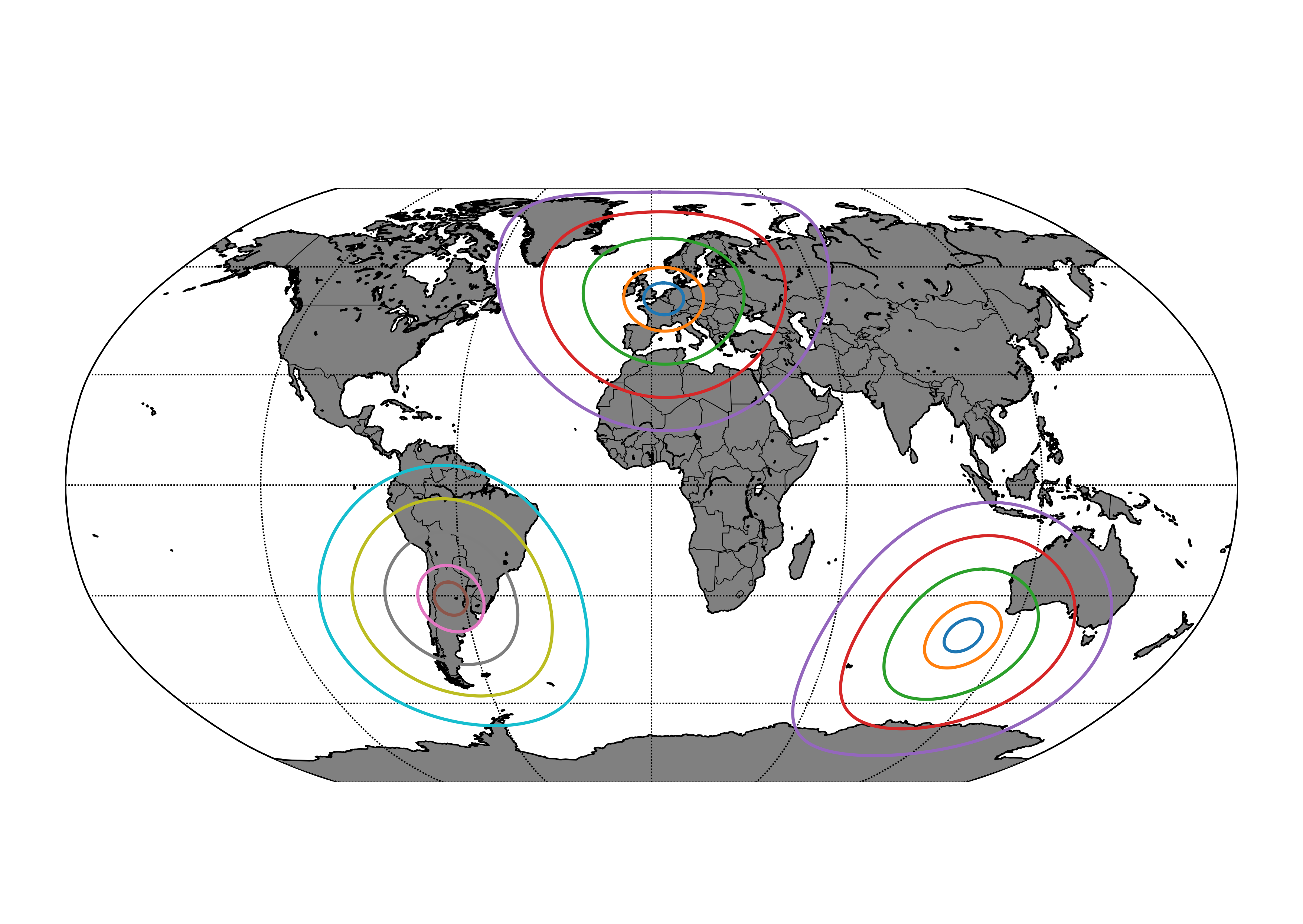

参考：

1.http://www.geophysique.be/2011/02/20/matplotlib-basemap-tutorial-09-drawing-circles/