计算神经元动力学编程模型Brainpy下载和测试

资源链接分享

B站的介绍
项目主页
github课程资料
Brainpy的模型代码示例

依赖的包JAX
JAX 是一个 Python 库，用于面向加速器的数组计算和程序转换，专为高性能数值计算和大规模机器学习而设计。

支撑文献

下载的页面

下载过程

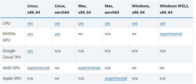
下载分为不同版本，brainpy主要依赖的包是JAX这个大规模数值计算的库。
支持cpu，gpu和tpu三种计算平台。支持的python版本是Python 3.9 - 3.11。

这里只写cpu和gpu版本的下载。

要安装只在 CPU 上运行的 BrainPy 版本（这可能对在笔记本电脑上进行本地开发很有用），可以运行

说明windows只支持cpu版本的，因为brainpy版本的支持高性能计算的jax库和jaxlib。

 pip install brainpy[cpu]

BrainPy 支持 SM 5.2 (Maxwell) 或更新版本的英伟达™（NVIDIA®）图形处理器。 要安装纯 GPU 版本的 BrainPy，可以运行

pip install brainpy[cuda12] -f https://storage.googleapis.com/jax-releases/jax_cuda_releases.html  # for CUDA 12.0
pip install brainpy[cuda11] -f https://storage.googleapis.com/jax-releases/jax_cuda_releases.html

根据cuda的版本自行下载。
使用conda 配置的命令如下：

conda create -n brainpy_gpu python=3.11

conda activate brainpy_gpu
#查看cuda版本
nvcc -V
#下载cuda12的版本
pip install brainpy[cuda12] -f https://storage.googleapis.com/jax-releases/jax_cuda_releases.html

示例代码中使用到matplotlib绘图，不知道上面那个库为什么没有涵盖。

#下载matplotlib
conda install matplotlib
#在执行代码时出现ImportError: Numba needs NumPy 2.0 or less. Got NumPy 2.1.
#版本要求numpy为之前的版本，重新下载老的版本。
pip install numpy==2.0

运行示例测试

环境设置

在vscode 中执行
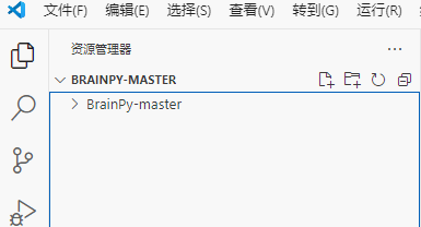
选择环境前要先打开对应的文件夹。
打开github下载的仓库

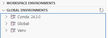
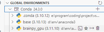
使用 Python Environment Manager 插件选择新创建的环境

点击星星选中

执行example中的几个例子：

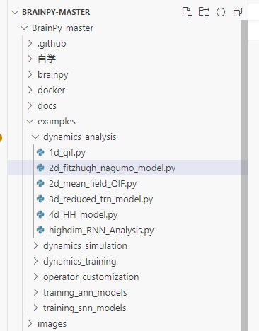
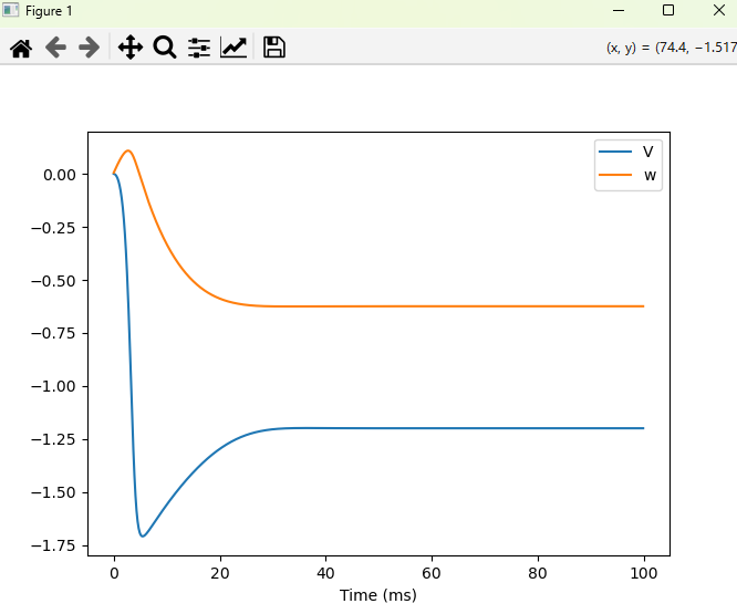
2d_fitzhugh_nagumo_model

# -*- coding: utf-8 -*-


import brainpy as bp
import brainpy.math as bm

bp.math.enable_x64()


class FitzHughNagumoModel(bp.DynamicalSystem):
  def __init__(self, method='exp_auto'):
    super(FitzHughNagumoModel, self).__init__()

    # parameters
    self.a = 0.7
    self.b = 0.8
    self.tau = 12.5

    # variables
    self.V = bm.Variable(bm.zeros(1))
    self.w = bm.Variable(bm.zeros(1))
    self.Iext = bm.Variable(bm.zeros(1))

    # functions
    def dV(V, t, w, Iext=0.):
      dV = V - V * V * V / 3 - w + Iext
      return dV

    def dw(w, t, V, a=0.7, b=0.8):
      dw = (V + a - b * w) / self.tau
      return dw

    self.int_V = bp.odeint(dV, method=method)
    self.int_w = bp.odeint(dw, method=method)

  def update(self):
    t = bp.share['t']
    dt = bp.share['dt']
    self.V.value = self.int_V(self.V, t, self.w, self.Iext, dt)
    self.w.value = self.int_w(self.w, t, self.V, self.a, self.b, dt)
    self.Iext[:] = 0.


model = FitzHughNagumoModel()

# simulation
runner = bp.DSRunner(model, monitors=['V', 'w'], inputs=['Iext', 0.])
runner.run(100.)

bp.visualize.line_plot(runner.mon.ts, runner.mon.V, legend='V')
bp.visualize.line_plot(runner.mon.ts, runner.mon.w, legend='w', show=True)

# phase plane analysis
pp = bp.analysis.PhasePlane2D(
  model=model,
  target_vars={'V': [-3, 3], 'w': [-1, 3]},
  pars_update={'Iext': 1.},
  resolutions=0.01,
)
pp.plot_vector_field()
pp.plot_nullcline(coords={'V': 'w-V'})
pp.plot_fixed_point()
pp.plot_trajectory(initials={'V': [0.], 'w': [1.]},
                   duration=100, plot_durations=[50, 100])
pp.show_figure()


# codimension 1 bifurcation
bif = bp.analysis.Bifurcation2D(
  model=model,
  target_vars={'V': [-3., 3.], 'w': [-1, 3.]},
  target_pars={'Iext': [-1., 2.]},
  resolutions={'Iext': 0.01}
)
bif.plot_bifurcation(num_par_segments=2)
bif.plot_limit_cycle_by_sim()
bif.show_figure()

代码目前还没开始看，先运行看看结果。

运行一个example中的例子：

Brainpy的模型代码示例

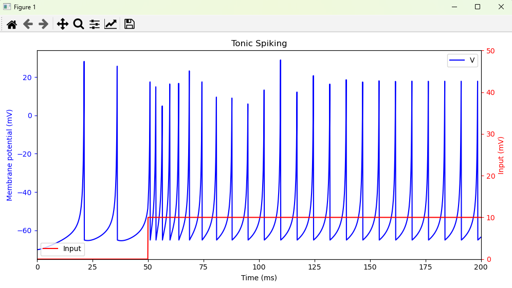
Tonic Spiking

import brainpy as bp

import matplotlib.pyplot as plt

neu = bp.neurons.Izhikevich(1)
neu.a, neu.b, neu.c, neu.d = 0.02, 0.40, -65.0, 2.0

current = bp.inputs.section_input(values=[0., 10.], durations=[50, 150])
runner = bp.DSRunner(neu, inputs=['input', current, 'iter'], monitors=['V', 'u'])
runner.run(duration=200.)

fig, ax1 = plt.subplots(figsize=(10, 5))
plt.title('Tonic Spiking')
ax1.plot(runner.mon.ts, runner.mon.V[:, 0], 'b', label='V')
ax1.set_xlabel('Time (ms)')
ax1.set_ylabel('Membrane potential (mV)', color='b')
ax1.set_xlim(-0.1, 200.1)
ax1.tick_params('y', colors='b')

ax2 = ax1.twinx()
ax2.plot(runner.mon.ts, current, 'r', label='Input')
ax2.set_xlabel('Time (ms)')
ax2.set_ylabel('Input (mV)', color='r')
ax2.set_ylim(0, 50)
ax2.tick_params('y', colors='r')
ax1.legend(loc=1)
ax2.legend(loc=3)
fig.tight_layout()
plt.show()

下一步计划

github课程资料
在这个里面的PPT中，学习一下课程，结合chatgpt进行学习