


文章目录
人工智能的三个学派
人工智能:让机器具备人的思维和意思
行为主义
- 基于控制论,构建
感知-动作控制系统 - 控制论,如平衡、行走、避障等自适应控制系统
符号主义
- 基于算数逻辑表达式,求解问题时先把问题描述为表达式,再求解表达式
- 可用公式描述、实现理性思维,如专家系统
连接主义(主流)
- 仿生学,模仿神经元连接关系
- 仿脑神经元连接,实现感性思维,如神经网络
随着我们的成长,大量的数通过视觉、听觉涌入大脑,使我们神经元连接线上的权重发生了变化
用计算机仿出神经网络连接关系
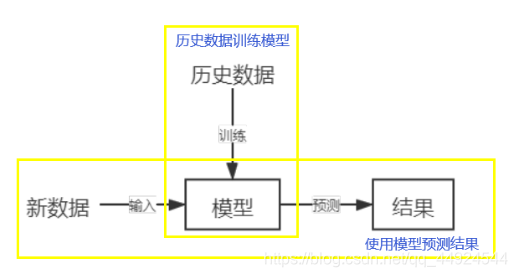
- 准备数据:采集大量 ”特征/标签“ 数据
- 搭建网络:搭建神经网络结构
- 优化参数:训练网络获取最佳参数(反转)
- 应用网络:将网络保存为模型,输入新数据,输出分类或预测结果(前传)
神经元的计算模型(MP模型)
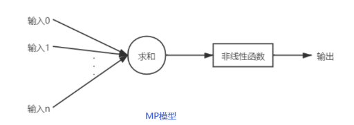
- 非线性函数,也就是激活函数
前向传播
- 输入x(输入特征和特征标签),执行MP模型,计算出y(输出),该过程就叫前向传播
损失函数
- 损失函数:定义y(预测值)与y_(标准答案)的差距
- 损失函数可以定量判断W(权重)、b(偏置值)的优劣
- 当损失函数输出最小时,参数W、b会出现最优值
- 均方误差:MSE(y, y_)= ∑ k = 0 n ( y − y _ ) 2 n \frac{\sum_{k=0}^{n}{(y-y\_)^2}}{n} n∑k=0n(y−y_)2
梯度下降
- 目的:找到一组参数w和b,使得损失函数最小
- 梯度:函数对各参数求偏导后的向量,函数梯度下降方向是函数的减小方向
- 梯度下降法:沿损失函数梯度下降的方向,寻找损失函数的最小值,得到最优参数的方法
- 梯度的计算方式是求解函数关于每个变量的一阶偏导
- 梯度的标记为▽
- 梯度是个向量
- 梯度表示函数变化率最快最大的方向
学习率
- 当学习率设置过小,收敛过程将变得十分缓慢·
- 当学习率设置过大,梯度可能会在最小值附近来回振荡,甚至可能无法收敛
反向传播
从后向前,逐层求损失函数对每层神经元参数的偏导数,迭代更新所有参数
w t + 1 = w t − l r ∗ ∂ l o s s ∂ w t w_{t+1}=w_t-lr*\frac{\partial loss}{\partial w_t} wt+1=wt−lr∗∂wt∂loss
import tensorflow as tf

w = tf.Variable(tf.constant(5, dtype=tf.float32))
lr = 0.2  # 学习率
epochs = 40

# 对数据集循环epoch次, 此例数据集数据仅有1个w, 设置随机初始值为5,循环40次迭代
for epoch in range(epochs):
    with tf.GradientTape() as tape:  # with结构到grads框起了梯度的计算过程
        loss = tf.square(w + 1)  # 损失函数
    grads = tape.gradient(loss, w)  # gradient函数告知谁对谁求导

    # assign_sub 对变量做自减 即:w -= lr*grads 即 w = w - lr*grads
    w.assign_sub(lr * grads)

    print("After %s epoch, w is %f, loss is %f" % (epoch, w.numpy(), loss))

# lr初始值:0.2   请自改学习率  0.001  0.999 看收敛过程
# 最终目的:找到 loss 最小 即 w = -1 的最优参数w
张量
概念
- 张量(Tensor):多维数组(列表),阶:张量的维数
- 张量可以表示0阶到n阶数组(列表)
- 0阶张量是标量,表示一个单独的数
- 1阶张量是向量,表示一个单独的数
- 2阶张量是矩阵,表示的是二维矩阵
数据类型
- tf.int
- tf.int32
- tf.int64
- tf.float
- tf.float32
- tf.float64
- tf.bool
- tf.constant([True, False])
- tf.string
- tf.constant(“Hello, world!”)
创建张量
-
tf.constant(张量内容, dtype=数据类型(可选))
import tensorflow as tf
a = tf.constant([1, 5], dtype=tf.int64)

print(a)
print(a.dtype)
print(a.shape)

# 运行结果
tf.Tensor([1 5], shape=(2,), dtype=int64)
<dtype: 'int64'>
(2,)
创建特殊张量
-
tf.zeros(维度):创建全为0的张量
import tensorflow as tf a = tf.zeros([2, 3]) -
tf.ones(维度):创建全为1的张量
import tensorflow as tf b = tf.ones(4) -
tf.fill(维度, 指定值):创建全为指定值的张量
import tensorflow as tf
c = tf.fill([2, 3, 4], 6)
创建符合正态分布的张量
- tf.random.normal(维度, mean=均值, stddev=标准差)
- 符合正太分布的随机数
- 默认均值为0,标准差为1
- tf.random.truncated_normal(维度, mean=均值, stddev=标准差)
- 符合正太分布的随机数
- 默认均值为0,标准差为1
- 数据在μ ±2 σ之间
生成均匀分布随机数
-
tf.random.uniform(维度, minval=最小值, maxval=最大值)
import tensorflow as tf
f = tf.random.uniform([2, 2], minval=0, maxval=1)
转换张量
-
tf.convert_to_tensor(数据名, dtype=数据类型(可选))
import tensorflow as tf
import numpy as np
a = np.arrange(0, 5)
b = tf.convert_to_tensor(a, dtype=tf.int64)
常用函数
强制类型转换
- tf.cast(张量名, dtype=数据类型)
计算张量维度上元素的最值
- tf.reduce_min(张量名, axis=操作轴)
- tf.reduce_max(张量名, axis=操作轴)
- tf.reduce_mean(张量名, axis=操作轴):计算张量沿着指定维度的平均值
- tf.reduce_sum(张量名, axis=操作轴):计算张量沿着指定维度的和
- 不指定axis,则对所有元素进行操作
理解axis
- axis = 0 表示对第一个维度进行操作
- axis = 1 表示对第二个维度进行操作
标记函数
-
tf.Variable(初始值)
- 将标量标记为“可训练”
- 被标记的变量会在反向传播中记录梯度信息
- 神经网络训练中,常用该函数标记待训练参数
import tensorflow as tf
w = tf.Variable(tf.random.normal([2, 2], mean=0, stddev=1))
数学运算
四则远算
只由维度相同的张量才可以进行四则远算
- tf.add(张量1, 张量2):加
- tf.subtract(张量1, 张量2):减
- tf.multiply(张量1, 张量2):乘
- tf.divide(张量1, 张量2):除
矩阵运算
- tf.square(张量名):平方
- tf.pow(张量名, n次方):次方
- tf.sqrt(张量名):开方
- tf.matmul(矩阵1, 矩阵2):矩阵乘
- 两个矩阵中数据的类型应一致
特征标签配对函数
-
tf.data.Dataset.from_tensor_slices((输入特征, 标签))
- 切分传入张量第一维度,生成数据特征/标签对
- Numpy和Tensor格式都可用该语句读入数据
import tensorflow
features = tf.constant([12, 23, 10, 17])
labels = tf.constant([0, 1, 1, 0])
dataset = tf.data.Dataset.from_tensor_slices((features, labels))
求导
-
tf.GradientTape():
-
eager模式下计算梯度
-
实现某个函数对指定参数的求导计算
-
with结构记录计算过程,gradient求出张量的梯度
-
GradientTape也可以嵌套多层用来计算高阶导数
with tf.GradientTape() as tape:
    若干计算过程
grade = tape.gradient(函数, 对谁求导)
import tensorflow as tf with tf.GradientTape() as tape: w = tf.Variable(tf.constant(3.0)) loss = tf.pow(w, 2) grade = tape.gradient(loss, w) print(grade) -
枚举
- enumerate
- Python内置函数
- 遍历每个元素
- 组合为:索引 元素
- 常在for循环中使用
独热码
- 独热编码(one-hot encoding)
- 在分类问题中,常用独热码做标签
- 标记类别:1表示是,0表示非
-
tf.one_hot(待转换数据, depth=几分类)
- 将待转换数据转换为one-hot形式的数据输出
import tensorflow as tf classes = 3 labels = tf.constant([1, 0, 2]) # 鸢尾花分类,输入元素值最小为0,最大为2 output = tf.one_hot(labels, depth=classes) print(output)tf.Tensor( [[0. 1. 0.] [1. 0. 0.] [0. 0. 1.]], shape=(3, 3), dtype=float32)
参数自更新
-
assign_sub()
- 赋值操作,更新参数的值并返回
- 调用assign_sub()之前,先用tf.Variable()定义变量w为可训练(可自更新)
- w.assign_sub(w要自减的内容)
import tensorflow as tf
w = tf.Variable(4)
w.assign_sub(1) # w = w-1
print(w)

运行结果:
<tf.Variable 'Variable:0' shape=() dtype=int32, numpy=3>
tf.nn.softmax()
Softmax( y i y_i yi) = e y i ∑ j = 0 n e y i \Large \frac{e^{y_i}}{\sum_{j=0}^{n}{e^{y_i}}} ∑j=0neyieyi
-
使输出符合概率分布
-
当n分类的n个输出(y0, y1, … yn-1)通过softmax()函数,便符合概率分布了
import tensorflow as tf
y = tf.constant([1.01, 2.01, -0.66])
y_pro = tf.nn.softmax(y)
print("After softmax, y_pro is", y_pro)

# 运行结果
After softmax, y_pro is tf.Tensor([0.25598174 0.69583046 0.0481878 ], shape=(3,), dtype=float32)
tf.argmax(张量名, axis=操作轴)
- 返回张量沿指定维度最大值的索引
import tensorflow as tf
import numpy as np
test = np.array([[1, 2, 3], [2, 3, 4], [5, 4, 3], [8, 7, 2]])
print(test)
print(tf.argmax(test, axis=0)) # 返回每一列(经度)最大值的索引
print(tf.argmax(test, axis=1)) # 返回每一行(经度)最大值的索引

运行结果:
[[1 2 3]
 [2 3 4]
 [5 4 3]
 [8 7 2]]
tf.Tensor([3 3 1], shape=(3,), dtype=int64)
tf.Tensor([2 2 0 0], shape=(4,), dtype=int64)
神经网络实现鸢尾花分类
准备数据
-
数据集读入
# 从sklearn包datasets读入数据集 from sklearn import datasets x_data = datasets.load_iris().data # data返回iris数据集所有输入特征 y_data = datasets.load_iris().target # target返回iris数据集所有标签 -
数据集乱序
np.random.seed(116) # 使用相同的seed,使输入特征/标签一一对应 np.random.shuffle(x_data) np.random.seed(116) np.random.shuffle(y_data) np.random.seed(116) -
生成训练集和测试集(即x_train/y_train, x_test/y_test)
x_train = x_data[:-30] y_train = y_data[:-30] x_test = x_data[-30:] y_test = x_data[-30:] -
配成(输入特征,标签)对,每次读入一小撮(batch)
train_db = tf.data.Dataset.from_tensor_slices((x_train, y_train)).batch(32)
test_db = tf.data.Dataset.from_tensor_slices((x_test, y_test)).batch(32)
搭建网络
-
定义神经网络中所有可训练参数
- 4个输入特征,故输入层为4个输入节点;因为3分类,故输出层为3个神经元
- 使用seed使每次生成的随机数相同,现实使用时不写seed
w1 = tf.Variable(tf.random.truncated_normal([4, 3], stddev=0.1, seed=1))
b1 = tf.Variable(tf.random.truncated_normal([3], stddev=0.1, seed=1))
参数优化
-
嵌套循环迭代,with结构更新参数,显示当前loss
for epoch in range(ephochs): # 数据集级别迭代
    for step, (x_train, y_train) in enumerate(train_db): # batch级别迭代
        with tf.GradientTape() as tape: # 记录梯度细腻
            前向传播过程计算y
            计算总loss
        grads = tape.gradient(loss, [w1, b1])
        w1.assign_sub(lr * grades[0]) # 参数自更新
        b1.assign_sub(lr * grades[1])
    print("Epoch {}, loss: {}".format(epoch, loss_all/4))
测试效果
-
计算当前参数前向传播后的准确率,显示当前acc(准确率)
for x_test, y_test in test_db:
    y = tf.matmul(x_test, w1) + b # y为预测结果
    y = tf.nn.softmax(y) # y符合概率分布
    pred = tf.argmax(y, axis=1) # 返回y中最大值的索引,即预测的分类
    pred = tf.cast(pred, dtype=y_lest.dtype) # 调整数据类型与标签一致
    correct = tf.cast(tf.equal(pred, y_test), dtype=tf.int32)
    correct = tf.reduce_sum(correct) # 将每个batch的correct数加起来
    total_correct += int(correct) # 将所有batch中得correct数加起来
    total_number += x_test.shape[0]
acc = total_correct / total_number
print("test_acc", acc)
acc/loss可视化
plt.title("Acc Curve") # 图片标题
plt.xlabel("Epoch") # x轴名称
plt.ylabel("Acc") # y轴名称
plt.plot(test_acc, label="$Accuracy$") # 逐步画出test_acc值并连线
plt.legend()
plt.show()


 被折叠的 条评论
为什么被折叠?
被折叠的 条评论
为什么被折叠?
 到【灌水乐园】发言


