


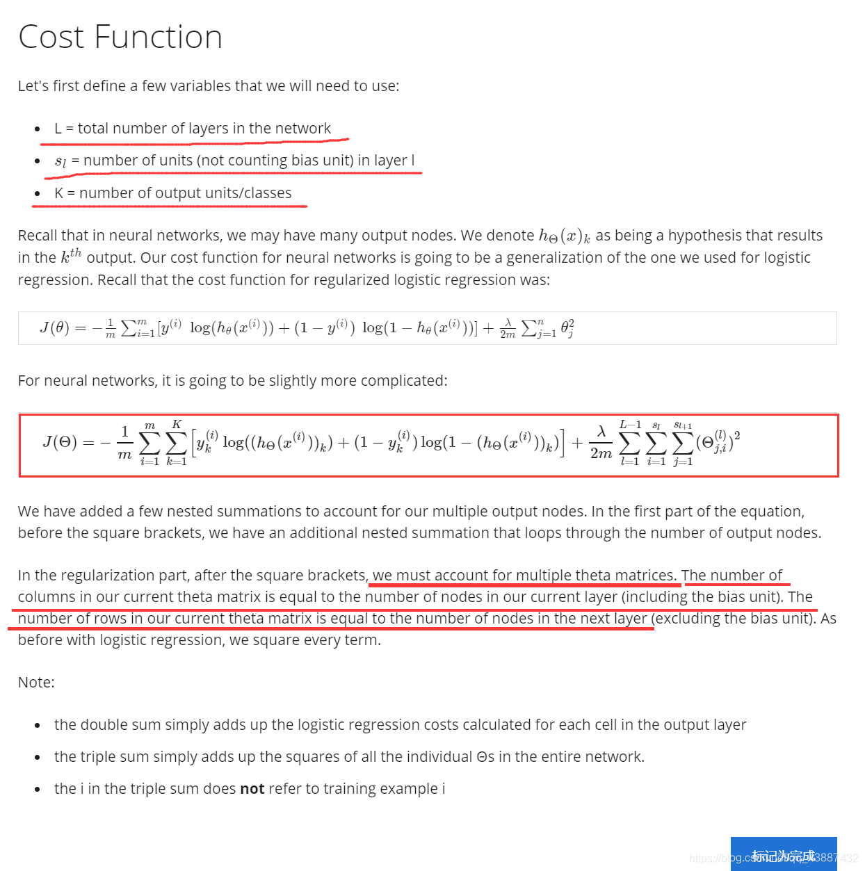
反向传播算法
反向传播是神经网络中的一个术语,利用反向传播可以最小化代价函数。类似在线性回归和逻辑回归中,利用梯度下降所做的工作,在神经网络中,我们的目的也是计算
m
i
n
θ
J
(
θ
)
min_\theta J(\theta)
minθJ(θ),也就是想要找到一组最优的参数
θ
\theta
θ来最小化我们的代价函数。
反向传播的算法如下:
训练集为 ( x ( 1 ) , y ( 1 ) ) , . . . ( x ( m ) , y ( m ) ) {(x^{(1)},y^{(1)})},...(x^{(m)},y^{(m)}) (x(1),y(1)),...(x(m),y(m))
Set Δ i j ( l ) = 0 \Delta_{ij}^{(l)} = 0 Δij(l)=0(for all i, j, l)
For i = 1 to m
(缩进) Set a ( 1 ) = x ( i ) a^{(1)}=x^{(i)} a(1)=x(i)
(缩进)Perform forward propagation to compute a ( l ) a^{(l)} a(l) for l = 2 , 3 , 4 , . . . L l=2,3,4,...L l=2,3,4,...L
(缩进)Using y ( i ) y^{(i)} y(i), compute δ ( L ) = a ( L ) − y ( i ) \delta^{(L)}=a^{(L)}-y^{(i)} δ(L)=a(L)−y(i)
(缩进)Compute δ ( L − 1 ) , δ ( L − 2 ) , . . . δ ( 2 ) \delta^{(L-1)},\delta^{(L-2)},...\delta^{(2)} δ(L−1),δ(L−2),...δ(2)
(缩进) Δ i j ( l ) : = Δ i j ( l ) + a j ( l ) δ i ( l + 1 ) \Delta^{(l)}_{ij}:=\Delta^{(l)}_{ij}+a^{(l)}_j\delta^{(l+1)}_i Δij(l):=Δij(l)+aj(l)δi(l+1)
D i j ( l ) : = 1 m Δ i j ( l ) + λ θ i j ( l ) i f j ≠ 0 D_{ij}^{(l)}:=\frac{1}{m}\Delta_{ij}^{(l)}+\lambda\theta_{ij}^{(l)} if j \neq 0 Dij(l):=m1Δij(l)+λθij(l)ifj=0
D i j ( l ) : = 1 m Δ i j ( l ) i f j = 0 D_{ij}^{(l)}:=\frac{1}{m}\Delta_{ij}^{(l)} if j = 0 Dij(l):=m1Δij(l)ifj=0
//D就是J对 θ \theta θ的导数
如何计算 δ \delta δ
δ
(
L
)
=
a
(
L
)
−
y
(
t
)
\delta^{(L)}=a^{(L)}-y^{(t)}
δ(L)=a(L)−y(t)(L表示神经网络的层数。神经网络中最后一层的误差就是预测值和实际值之间的误差)
之后按照
L
−
1
,
L
−
2
,
L
−
3
,
.
.
.
2
L-1,L-2,L-3,...2
L−1,L−2,L−3,...2的顺序计算
δ
\delta
δ
δ
(
l
)
=
(
(
θ
(
l
)
)
T
δ
(
l
+
1
)
.
∗
a
(
l
)
.
∗
(
1
−
a
(
l
)
)
\delta^{(l)}=((\theta^{(l)})^{T} \delta^{(l+1)}.*a^{(l)}.*(1-a^{(l)})
δ(l)=((θ(l))Tδ(l+1).∗a(l).∗(1−a(l))
梯度检测
为了检验反向传播算法是否正确,可以借助梯度检测进行验证。编写反向传播时将其结果和梯度检测得到的结果进行比较,来检验反向传播编写是否正确。但是实际训练网络时,需要将梯度检测关闭,因为梯度检测的代价很大。
∂
∂
θ
j
J
(
θ
)
≈
J
(
θ
+
ϵ
)
−
J
(
θ
−
ϵ
)
2
ϵ
\frac{\partial}{\partial\theta_j}J(\theta)\approx\frac{J(\theta+\epsilon)-J(\theta-\epsilon)}{2\epsilon}
∂θj∂J(θ)≈2ϵJ(θ+ϵ)−J(θ−ϵ)
当
θ
\theta
θ是向量的时候,得到:
∂
∂
θ
j
J
(
θ
)
≈
J
(
θ
1
,
.
.
.
,
θ
j
+
ϵ
,
.
.
.
,
θ
n
)
−
J
(
θ
1
,
.
.
.
,
θ
j
−
ϵ
,
.
.
.
,
θ
n
)
2
ϵ
\frac{\partial}{\partial\theta_j}J(\theta)\approx\frac{J(\theta_1,...,\theta_j+\epsilon,...,\theta_n)-J(\theta_1,...,\theta_j-\epsilon,...,\theta_n)}{2\epsilon}
∂θj∂J(θ)≈2ϵJ(θ1,...,θj+ϵ,...,θn)−J(θ1,...,θj−ϵ,...,θn)
这里的
ϵ
\epsilon
ϵ选取要小(例如
ϵ
=
1
0
−
4
\epsilon=10^{-4}
ϵ=10−4),这样得到的结果才接近真实的导数值。
当反向传播得到的结果和梯度检测的结果是近似刻意看做相等的,则有理由相信反向传播算法是正确的。
随机初始化
在神经网络中,将
θ
\theta
θ初始化为0或者其他的相同的数字,是不会起作用的。所以要进行随机初始化。一种方法如下:
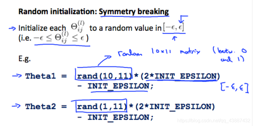
这样可以使
θ
i
j
(
l
)
\theta_{ij}^{(l)}
θij(l)均介于
[
−
ϵ
,
ϵ
]
[-\epsilon,\epsilon]
[−ϵ,ϵ]之间。
编程作业
checkNNGradients.py
from debugInitializeWeights import *
from nnCostFunction import *
from computeNumericalGradient import *
from numpy import linalg as la
from numpy import max

def checkNNGradients(my_lambda):
# CHECKNNGRADIENTS Creates a small neural network to check the
# backpropagation gradients
# CHECKNNGRADIENTS(lambda ) Creates a small neural network to check the
# backpropagation gradients, it will output the analytical gradients
# produced by your backprop code and the numerical gradients(computed
# using computeNumericalGradient).These two gradient computations should
# result in very similar values

    input_layer_size = 3
    hidden_layer_size = 25
    num_labels = 3
    m = 6

    # We generate some 'random' test data
    Theta1 = debugInitializeWeights(hidden_layer_size, input_layer_size) ##(25,3)
    Theta2 = debugInitializeWeights(num_labels, hidden_layer_size) ##(3,26)
    # Reusing debugInitializeWeights to generate X
    X  = debugInitializeWeights(m, input_layer_size - 1)##(6,3)
    y  = 1 + np.mod(np.arange(1, m + 1), num_labels)
    # Unroll parameters
    nn_params = np.append(Theta1, Theta2)

    # Short hand for cost function


    def cost_func(p):
        return nnCostFunction(p, input_layer_size, hidden_layer_size, num_labels, X, y, my_lambda)
    cost, grad = cost_func(nn_params)
    numgrad = computeNumericalGradient(nn_params, input_layer_size, hidden_layer_size, num_labels, X, y, my_lambda)

    # Visually examine the two gradient computations.  The two columns
    # you get should be very similar.
    ans = np.c_[numgrad, grad]
    print(ans)
    print('The above two columns you get should be very similar.'
         '(Left-Your Numerical Gradient, Right-Analytical Gradient)')
    '''
    # Evaluate the norm of the difference between two solutions.
    # If you have a correct implementation, and assuming you used EPSILON = 0.0001
    # in computeNumericalGradient.m, then diff below should be less than 1e-9
    numgrad = numgrad.reshape((numgrad.size, -1))
    grad = grad.reshape((grad.size, -1))
    diff = la.svd(numgrad-grad)/la.svd(numgrad+grad)
    ##返回矩阵的一个范数,具体来说是矩阵最大奇异值
    print('If your backpropagation implementation is correct, then '
         'the relative difference will be small (less than 1e-9). '
         'Relative Difference: {}'.format(diff))
    '''
computeNumericalGradient.py
import numpy as np
from nnCostFunction import nnCostFunction

def computeNumericalGradient(nn_params, input_layer_size, hidden_layer_size, num_labels, X, y, my_lambda):
# COMPUTENUMERICALGRADIENT Computes the gradient using "finite differences"
# and gives us a numerical estimate of the gradient.
    e = 0.0001
    numgrad = np.zeros(nn_params.size)
    print(nn_params.size)
    print('计算中的数字{}'.format(numgrad.shape))
    for i in range(nn_params.size):
        perturb = np.zeros(nn_params.size)
        perturb[i] = e
        loss1, grad1 = nnCostFunction(nn_params - perturb, input_layer_size, hidden_layer_size, num_labels, X, y, my_lambda)
        loss2, grad2 = nnCostFunction(nn_params + perturb, input_layer_size, hidden_layer_size, num_labels, X, y, my_lambda)
        #Compute Numerical Gradient
        numgrad[i] = (loss2 - loss1) / (2 * e)
        perturb[i] = 0
    return numgrad
debugInitializeWeights.py
import numpy as np
def debugInitializeWeights(fan_out, fan_in):
#DEBUGINITIALIZEWEIGHTS Initialize the weights of a layer with fan_in
#incoming connections and fan_out outgoing connections using a fixed
#strategy, this will help you later in debugging
#   W = DEBUGINITIALIZEWEIGHTS(fan_in, fan_out) initializes the weights
#   of a layer with fan_in incoming connections and fan_out outgoing
#   connections using a fix set of values
#
#   Note that W should be set to a matrix of size(1 + fan_in, fan_out) as
#   the first row of W handles the "bias" terms
#

    # Set W to zeros
    W = np.zeros(fan_out * (fan_in + 1))

    # Initialize W using "sin", this ensures that W is always of the same
    # values and will be useful for debugging
    for i in range(W.size):
        W[i] = np.sin(i) / 10
    W = W.reshape(fan_out, fan_in + 1)
    return W
displayData.py
import numpy as np
import matplotlib.pyplot as plt

####不知道为啥这样写,这是一篇博客里面的,看了看和题目给的matlab代码近似,
####只是将matlab代码转换成python代码

####看了代码大致明白是怎么实现的了
####将数据向量还原成20*20的矩阵块,之后将其作为图像进行显示即可
def display_data(x):
    (m, n) = x.shape  # 100*400

    example_width = np.round(np.sqrt(n)).astype(int)  # 每个样本显示宽度 round()四舍五入到个位 并转换为int
    example_height = np.floor(n / example_width).astype(int)  # 每个样本显示高度  并转换为int

    # 设置显示格式 100个样本 分10行 10列显示
    display_rows = np.floor(np.sqrt(m)).astype(int)
    display_cols = np.ceil(m / display_rows).astype(int)

    # 待显示的每张图片之间的间隔
    pad = 1

    # 显示的布局矩阵 初始化值为-1
    display_array = - np.ones((pad + display_rows * (example_height + pad),
                               pad + display_cols * (example_width + pad)))

    # Copy each example into a patch on the display array
    curr_ex = 0
    for j in range(display_rows):
        for i in range(display_cols):
            if curr_ex > m:##表示样本数量,显示的样本数量不能多于m
                break

            # Copy the patch
            # Get the max value of the patch
            max_val = np.max(np.abs(x[curr_ex]))
            display_array[pad + j * (example_height + pad) + np.arange(example_height),
                          pad + i * (example_width + pad) + np.arange(example_width)[:, np.newaxis]] = \
                x[curr_ex].reshape((example_height, example_width)) / max_val ##这个max_val不知道有什么用,去掉之后图像看起来没什么变化
            curr_ex += 1

        if curr_ex > m:
            break

    # 显示图片
    plt.figure()
    plt.imshow(display_array, cmap='gray', extent=[-1, 1, -1, 1])
    plt.axis('off')
    plt.show()
ex4.py
import scipy.io as scio
import numpy as np
from displayData import display_data
from nnCostFunction import *
from randInitializeWeights import *
from checkNNGradients import *
## Machine Learning Online Class - Exercise 4 Neural Network Learning

## =========== Part 1: Loading and Visualizing Data =============
#  We start the exercise by first loading and visualizing the dataset.
#  You will be working with a dataset that contains handwritten digits.
#

# Load Training Data
print('Loading and Visualizing Data ...')

data = scio.loadmat('D:\课程相关\吴恩达机器学习\Andrew-NG-Meachine-Learning-master\Andrew-NG-Meachine-Learning'
                    '-master\machine-learning-ex4\machine-learning-ex4\ex4\ex4data1.mat')
X = data['X']
y = data['y'].flatten()
m = y.size

# Randomly select 100 data points to display
rand_indics = np.random.permutation(range(m))
sel = X[rand_indics[0:100], :]
display_data(sel)
input('Program paused. Press enter to continue.')


## ================ Part 2: Loading Parameters ================
# In this part of the exercise, we load some pre-initialized
# neural network parameters.

print('Loading Saved Neural Network Parameters ...')

# Load the weights into variables Theta1 and Theta2
Theta = scio.loadmat('D:\课程相关\吴恩达机器学习\Andrew-NG-Meachine-Learning-master\Andrew-NG-Meachine-Learnin'
                     'g-master\machine-learning-ex4\machine-learning-ex4\ex4\ex4weights.mat')
Theta1 = Theta['Theta1']
Theta2 = Theta['Theta2']
# Unroll parameters
nn_params = np.append(Theta1, Theta2)

## ================ Part 3: Compute Cost (Feedforward) ================
#  To the neural network, you should first start by implementing the
#  feedforward part of the neural network that returns the cost only. You
#  should complete the code in nnCostFunction.m to return cost. After
#  implementing the feedforward to compute the cost, you can verify that
#  your implementation is correct by verifying that you get the same cost
#  as us for the fixed debugging parameters.
#
#  We suggest implementing the feedforward cost *without* regularization
#  first so that it will be easier for you to debug. Later, in part 4, you
#  will get to implement the regularized cost.
#


#这部分检测没有正则化时计算的代价函数是否正确
print('Feedforward Using Neural Network ...')
# Weight regularization parameter (we set this to 0 here).
my_lambda = 0
## Setup the parameters you will use for this exercise
input_layer_size  = 400   # 20x20 Input Images of Digits
hidden_layer_size = 25    # 25 hidden units
num_labels = 10           # 10 labels, from 1 to 10
                          # (note that we have mapped "0" to label 10)
J = nnCostFunction(nn_params, input_layer_size, hidden_layer_size, num_labels, X, y, my_lambda)[0]

print('Cost at parameters (loaded from ex4weights): {} (this value should be about 0.287629)'.format(J))

input('Program paused. Press enter to continue.')


## =============== Part 4: Implement Regularization ===============
#  Once your cost function implementation is correct, you should now
#  continue to implement the regularization with the cost.
#

print('Checking Cost Function (w/ Regularization) ... ')

# Weight regularization parameter (we set this to 1 here).
my_lambda = 1

J = nnCostFunction(nn_params, input_layer_size, hidden_layer_size, num_labels, X, y, my_lambda)[0]

print('Cost at parameters (loaded from ex4weights): {} (this value should be about 0.383770)'.format(J))

input('Program paused. Press enter to continue.')


## ================ Part 5: Sigmoid Gradient  ================
#  Before you start implementing the neural network, you will first
#  implement the gradient for the sigmoid function. You should complete the
#  code in the sigmoidGradient.m file.
#

print('Evaluating sigmoid gradient...')

g = sigmoidGradient(np.array([-1, -0.5, 0, 0.5, 1]))
print('Sigmoid gradient evaluated at [-1 -0.5 0 0.5 1]:{}'.format(g))


input('Program paused. Press enter to continue.')


## ================ Part 6: Initializing Pameters ================
#  In this part of the exercise, you will be starting to implment a two
#  layer neural network that classifies digits. You will start by
#  implementing a function to initialize the weights of the neural network
#  (randInitializeWeights.m)

print('Initializing Neural Network Parameters ...')

initial_Theta1 = randInitializeWeights(input_layer_size, hidden_layer_size)
initial_Theta2 = randInitializeWeights(hidden_layer_size, num_labels)
# Unroll parameters
initial_nn_params = np.append(initial_Theta1, initial_Theta2)

'''
## =============== Part 7: Implement Backpropagation ===============
#  Once your cost matches up with ours, you should proceed to implement the
#  backpropagation algorithm for the neural network. You should add to the
#  code you've written in nnCostFunction.m to return the partial
#  derivatives of the parameters.
#
print('Checking Backpropagation... ')

#  Check gradients by running checkNNGradients
input('Program paused. Press enter to continue.')

## =============== Part 8: Implement Regularization ===============
#  Once your backpropagation implementation is correct, you should now
#  continue to implement the regularization with the cost and gradient.
#

print('Checking Backpropagation (w/ Regularization) ... ')

#  Check gradients by running checkNNGradients
my_lambda = 3
checkNNGradients(my_lambda)
'''

my_lambda = 3

# Also output the costFunction debugging values
debug_J = nnCostFunction(nn_params, input_layer_size,
                          hidden_layer_size, num_labels, X, y, my_lambda)[0]

print('Cost at (fixed) debugging parameters (w/ lambda = {}):'.format(my_lambda))
print('{}(for lambda = 3, this value should be about 0.576051)'.format(debug_J))

input('Program paused. Press enter to continue.')

## =================== Part 8: Training NN ===================
#  You have now implemented all the code necessary to train a neural
#  network. To train your neural network, we will now use "fmincg", which
#  is a function which works similarly to "fminunc". Recall that these
#  advanced optimizers are able to train our cost functions efficiently as
#  long as we provide them with the gradient computations.
#
print('Training Neural Network... ')

#  After you have completed the assignment, change the MaxIter to a larger
#  value to see how more training helps.


#  You should also try different values of lambda
mld = 1
# Create "short hand" for the cost function to be minimized
def costFunction(p):
    return nnCostFunction(p, input_layer_size, hidden_layer_size, num_labels, X, y, mld)[0]
def gradFunction(p):
    return nnCostFunction(p, input_layer_size, hidden_layer_size, num_labels, X, y, mld)[1]
# Now, costFunction is a function that takes in only one argument (the neural network parameters)
from scipy.optimize import fmin_cg
#nn_params, cost, *unused = fmin_cg(f=costFunction, fprime=gradFunction,
  #                                   x0=initial_nn_params, full_output=True, disp=False,maxiter=50)
'''
input_layer_size  = 400   # 20x20 Input Images of Digits
hidden_layer_size = 25    # 25 hidden units
num_labels = 10           # 10 labels, from 1 to 10
'''

#nn_params = fmin_cg(f=costFunction, fprime=gradFunction, x0=initial_nn_params, maxiter=50, disp=True, full_output=True)

nn_params = fmin_cg(costFunction, fprime=gradFunction, x0=initial_nn_params, maxiter=50, disp=True)
# Obtain Theta1 and Theta2 back from nn_params
Theta1 = nn_params[:(input_layer_size + 1) * hidden_layer_size].reshape((hidden_layer_size, (input_layer_size + 1)))

Theta2 = nn_params[(input_layer_size + 1) * hidden_layer_size:].reshape((num_labels, (hidden_layer_size + 1)))

input('Program paused. Press enter to continue.')


## ================= Part 9: Visualize Weights =================
#  You can now "visualize" what the neural network is learning by
#  displaying the hidden units to see what features they are capturing in
#  the data.

print('Visualizing Neural Network... ')

display_data(Theta1[:, 1:])

input('Program paused. Press enter to continue.')

## ================= Part 10: Implement Predict =================
#  After training the neural network, we would like to use it to predict
#  the labels. You will now implement the "predict" function to use the
#  neural network to predict the labels of the training set. This lets
#  you compute the training set accuracy.

from predict import *
pred = predict(Theta1, Theta2, X)

print('Training Set Accuracy: {}'.format(np.mean(pred == y) * 100))
nnCostFunction.py
import numpy as np

def h(theta, X):
    X = np.c_[np.ones(X.shape[0]), X]
    z = np.dot(X, theta.T)
    return 1 / (1 + np.exp(-z))

def sigmoid(z):
    return 1 / (1 + np.exp(-z))

def sigmoidGradient(z):
    g = sigmoid(z)
    return g * (1 - g)
##y的标签是10,9,8,7,...1
def nnCostFunction(nn_params, input_layer_size, hidden_layer_size, num_labels, X, y, my_lambda):
    # =========your code here=======
    #instructions: you should complete the code by working through the following parts
    #Part1:feedforward the neural network ans return the cost in the variable J.
    Theta1 = nn_params[:(input_layer_size + 1) * hidden_layer_size].reshape((hidden_layer_size, (input_layer_size + 1)))
    Theta2 = nn_params[(input_layer_size + 1) * hidden_layer_size:].reshape((num_labels, (hidden_layer_size + 1)))
    # Setup some useful variables
    m = y.size
    a2 = h(Theta1, X)
    a3 = h(Theta2, a2)  # 这个就是输出的预测结果
    ##将标签变成矩阵形式
    Y = np.zeros((m, num_labels))
    for i in range(m):
        Y[i, y[i] - 1] = 1

    ##没有正则化的代价函数
    #J = -1 / m * np.sum(np.multiply(Y, np.log(a3)) + np.multiply(1 - Y, np.log(1 - a3)))

    ##theta中和X新加的1那列相乘的部分不用正则化
    reg_theta1 = Theta1[:, 1:]
    reg_theta2 = Theta2[:, 1:]
    ##正则化之后的代价函数,取my_lambda是0,就是没有正则化的代价函数
    ##这个代价函数和计算grad是没有直接关系的
    J = -1 / m * np.sum(np.multiply(Y, np.log(a3)) + np.multiply(1 - Y, np.log(1 - a3))) + my_lambda / (2 * m) * (np.sum(
        np.multiply(reg_theta1, reg_theta1)) + np.sum(np.multiply(reg_theta2, reg_theta2)))
    #cost function
    #Part2: Implement the backpropagation algorithm to compute the gradients
    #Theta1_grad and Theta2_grad.You should return the partial derivatives of
    #the cost function with respect to Theta1 and Theta2 in Theta1_grad and
    #Theta2_grad, respectively.After implementing Part 2, you can check
    #that your implementation is correct by running checkNNGradients

#Note: The vector y passed into the function is a vector of labels
#               containing values from 1..K. You need to map this vector into a
#               binary vector of 1's and 0's to be used with the neural network
#               cost function.
#
#         Hint: We recommend implementing backpropagation using a for-loop
#               over the training examples if you are implementing it for the
#               first time.

    #a2和a3已经计算出来了
    a2 = np.c_[np.ones(a2.shape[0]), a2]
    delta3 = a3 - Y ##5000*10
    delta2 = np.dot(delta3, Theta2) * a2 * (1 - a2) ##5000*26
    ##去掉第一列
    delta2 = delta2[:, 1:] ##5000*25
    X = np.c_[np.ones(X.shape[0]), X]
    Delta1 = np.dot(delta2.T, X) ##25, 401
    Delta2 = np.dot(delta3.T, a2) ##10, 26
    reg_Delta1 = my_lambda / m * np.c_[np.zeros(hidden_layer_size), reg_theta1]
    reg_Delta2 = my_lambda / m * np.c_[np.zeros(num_labels), reg_theta2]
    grad1 = (1 / m) * Delta1 + reg_Delta1
    grad2 = (1 / m) * Delta2 + reg_Delta2
    grad = np.append(grad1, grad2)
    return J, grad
predict.py
import numpy as np
from nnCostFunction import h

##输出标签
def predict(Theta1, Theta2, X):
    a2 = h(Theta1, X)
    a3 = h(Theta2, a2)
    ans = np.argmax(a3, axis=1)  # 找出每一行最大概率所在的位置
    ans += 1
    return ans
randInitializeWeights.py
'''
import numpy as np
#RANDINITIALIZEWEIGHTS Randomly initialize the weights of a layer with L_in
#incoming connections and L_out outgoing connections
#   W = RANDINITIALIZEWEIGHTS(L_in, L_out) randomly initializes the weights
#   of a layer with L_in incoming connections and L_out outgoing
#   connections.
#
#   Note that W should be set to a matrix of size(L_out, 1 + L_in) as
#   the first column of W handles the "bias" terms
#


# ====================== YOUR CODE HERE ======================
# Instructions: Initialize W randomly so that we break the symmetry while
#               training the neural network.
#
# Note: The first column of W corresponds to the parameters for the bias unit
#
def randInitializeWeights(L_in, L_out):
    # You need to return the following variables correctly
    W = np.zeros((L_out, 1 + L_in))
    theta_init = 0.12
    ###这个取值是根据输入和输出层单元个数选取的,一个合适的选择是取sqrt(6)/(sqrt(L_in+L_out))
    return np.random.rand(L_out, L_in + 1) * (2 * theta_init) - theta_init
'''
import numpy as np


def randInitializeWeights(l_in, l_out):
    # You need to return the following variable correctly
    w = np.zeros((l_out, 1 + l_in))

    # ===================== Your Code Here =====================
    # Instructions : Initialize w randomly so that we break the symmetry while
    #                training the neural network
    #
    # Note : The first column of w corresponds to the parameters for the bias unit
    #
    ep_init = 0.08
    w = np.random.rand(l_out, 1 + l_in) * (2 * ep_init) - ep_init
    # ===========================================================

    return w


 被折叠的 条评论
为什么被折叠?
被折叠的 条评论
为什么被折叠?
 到【灌水乐园】发言


