PointNet: Deep Learning on Point Sets for 3D Classification and Segmentation 论文和代码详解

Paper

该文章发表于2017年的CVPR（Computer Vision and Pattern Recognition），文章链接：

PointNet: Deep Learning on Point Sets for 3D Classification and Segmentation

Abstract

在本文中，设计了一种新型的直接处理点云的神经网络，它很好地考虑了输入点的排列不变性。网络名为PointNet，为object classification, part segmentation, scene semantic parsing等应用程序提供了统一的体系结构。虽然简单，但PointNet是高效和有效的。

1. Introduction

PointNet需要尊重以下事实：1，点云只是点的集合，因此对其成员的排列（在集合中的顺序）是不变的，在网络计算中需要某些对称；2，刚性运动不变性。

PointNet只是得到了点云的features，具体的应用需要接后续的相应的网络。本文进行了三个实验，所以提供的代码里一共有三个网络模型，分别对应三个不同的实验。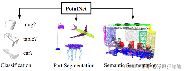

但是，这三个网络模型在由点云得到features的网络结构是相同的，这一部分正是本文的重点（贡献）所在。

3. Problem Statement

做的事情： 设计了一个能够直接处理以无序的点云作为输入的学习框架。

输入： 3D点云 { P i ∣ i = 1 , ⋯   , n } \{P_i|i=1,\cdots,n\} {Pi​∣i=1,⋯,n}，其中每个点$P_i$是一个由该点坐标$(x,y,z)$加额外feature channels构成的向量。本文为了简便，只用了点的坐标$(x,y,z)$作为点的channels。

输出： 对于分类任务，输出是对应 $k$ 个分类的 $k$ 个分数；对于语义分割任务，输出是$n\times m$个分数，对应于 $n$ 个点和 $m$ 个分割策略。

4. Deep Learning on Point Sets

4.1 Properties of Point Sets in $R^n$

1，无序性。 网络应该是关于点的输入顺序（对于$N$个点，有$N!$种顺序）是不变的。

2，点之间的相互作用。 点云中的点不是孤立的，一个点的邻域是有意义的子集。因此，网络需要能够从一个点的邻域捕捉局部特征以及这些局部结构之间的相互作用。但是，PointNet好像并不能捕捉一个点邻域的局部特征，PointNet++可以。

3，刚性运动不变性。 网络应该对点云的刚性变换不变。

4.2 PointNet Architecture

这一小节是重点！！！

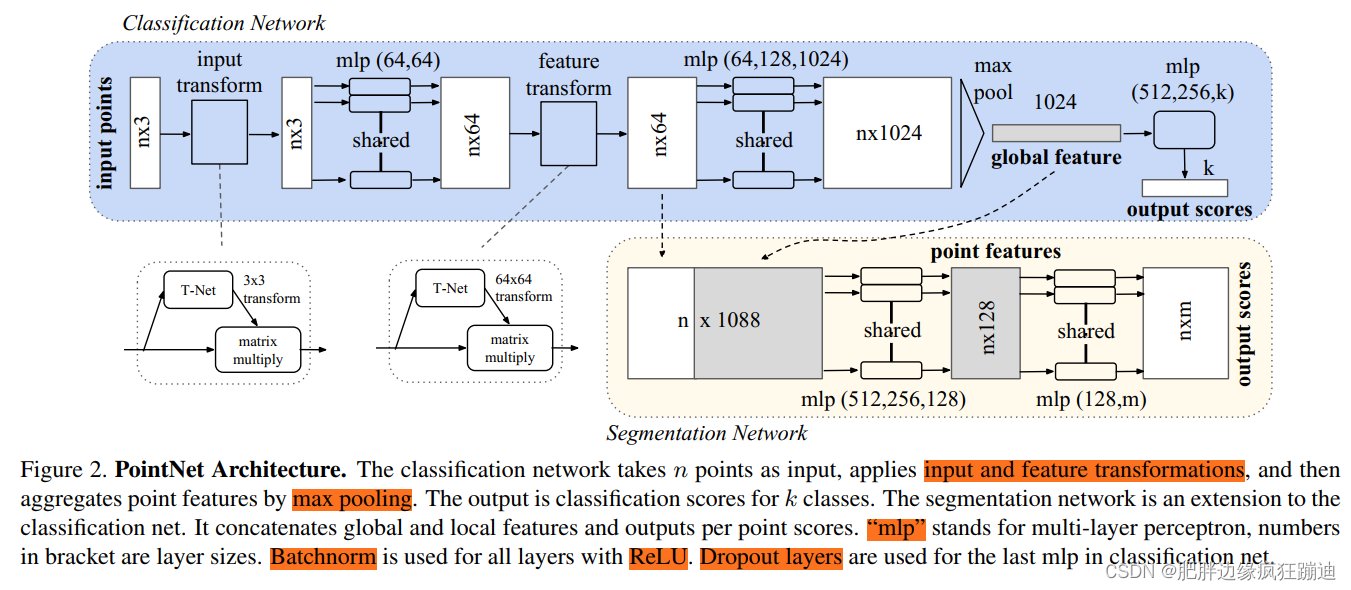
PointNet网络结构如下图所示：

input points： 输入是一个$n\times 3$的矩阵。（由于作者的代码实现是用卷积网络，所以可以将输入看为$n\times 3\times 1$的）

input transform： 生成一个$3\times 3$的变换矩阵，然后将该矩阵作用于输入点云。目的是对齐输入点云到一个标准空间。

shared mlp(64,64)： 共享权重的两层都是64个神经元的感知机。（此处的共享权重是指，因为每个点都是独立的，所以这些点的mlp是相同的，即一个，而不是$n$个。这也是用卷积网络来实现的原因：mlp相当于过滤器（卷积核），每层过滤器的数目就是mlp每层的神经元的数目。）目的是特征升维。

feature transform： 生成一个$64\times 64$的变换矩阵，然后将该矩阵作用于前面得到的点云特征。目的是对齐特征空间。

shared mlp(64,128,1024)： 共享权重的三层感知机，每层的神经元数目对应于括号中的数字。目的是特征升维。

max pool： 池化层，用的是最大池化。目的是提取全局特征。

mlp(512,256,k)： 全连接网络。目的是用来k分类。

Segmentation Network的输入： 将全局特征和局部特征整合起来。此处的局部特征是单个点的特征，没有考虑点附近的邻域

shared mlp(512,256,128)： 共享权重的三层感知机。目的是特征降维。

shared mlp(128,m)： 共享权重的两层感知机。目的是对于每个点输出m个分类的分数。

网络结构有三个关键模块：

Symmetry Function for Unordered Input（对于无序输入的对称函数）

为了使得模型是关于输入点云排序不变的，已知的有三种方法：（1）把输入整理成一个标准顺序（2）将输入视为一个序列用来训练RNN，但是通过所有的排序来补充训练数据（3）用一个简单的对称函数从每一个点聚集信息，对称函数以$n$个向量作为输入，输出一个输入顺序不变的新的向量，比如，加法操作和乘法操作就是对称函数。

本文的想法是通过对集合中变换后的元素应用对称函数来近似定义在点集上的一般函数：

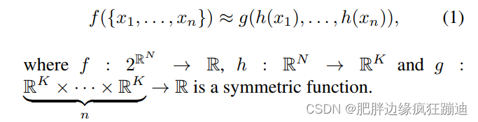
在本文中，用一个MLP近似 $h$，用一个单变量函数和一个最大池化函数的组合来近似 $g$。

Local and Global Information Aggregation（局部和全局信息聚合）

上一步的输出是形式为$[f_1,\cdots ,f_K]$的向量，这是输入集合的global feature。这个global feature可以直接接一个SVM或者MLP分类器用于classification。但是对于segmentation，需要a combination of local and global knowledge。所以，对于分割网络，如PointNet网络结构图所示，需要将global feature和local feature整合起来。

Joint Alignment Network（联合对齐网络）

通过一个微型网络(PointNet网络结构图中的T-net)预测两个仿射变换矩阵，一个是应用于输入点的坐标上的$3\times 3$矩阵，另一个是应用于点特征上的$64\times 64$矩阵。 微型网络本身类似于大网络，由点无关特征提取、最大池化和全连通层等基本模块组成。

因为点特征的变换矩阵维度太高，为了方便优化，在softmax training loss中加了一个正则项，将点特征变换矩阵约束为近似正交矩阵
$$L_{reg}=||I-A{A}^T|{|}_F^2$$

4.3 Theoretical Analysis

Universal approximation（通用逼近性）

这一部分对应于Symmetry Function for Unordered Input的理论分析：

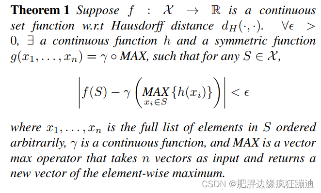
Bottleneck dimension and stability（瓶颈尺寸和稳定性）

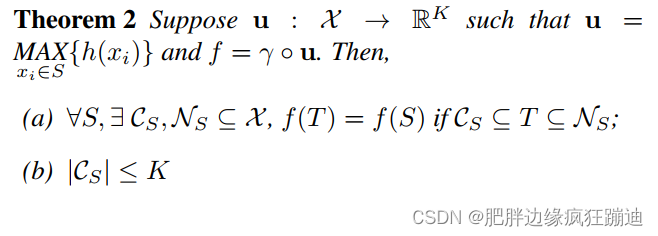
这条定理的解释如下：(a) says that $f(S)$ is unchanged up to the input corruption if all points in $C_S$ are preserved; it is also unchanged with extra noise points up to $N_S$. (b) says that $C_S$ only contains a bounded number of points, determined by $K$ in (1). In other words, $f(S)$ is in fact totally determined by a finite subset $C_S\subseteq S$ of less or equal to $K$ elements. Combined with the continuity of $h$, this explains the robustness of our model w.r.t point perturbation, corruption and extra noise points. Intuitively, our network learns to summarize a shape by a sparse set of key points. In experiment section we see that the key points form the skeleton of an object.

这条定理就是为了说明鲁棒性。

5. Experiment

5.1 Applications

3D Object Classification

数据集：ModelNet40。There are 12,311 CAD models from 40 man-made object categories, split into 9,843 for training and 2,468 for testing.

点云数目：We uniformly sample 1024 points on mesh faces according to face area and normalize them into a unit sphere. 每个模型的点云数目是一样的，并且是均匀分布的。

3D Object Part Segmentation

数据集：We evaluate on ShapeNet part data set, which contains 16,881 shapes from 16 categories, annotated with 50 parts in total. Most object categories are labeled with two to five parts. Ground truth annotations are labeled on sampled points on the shapes.

Semantic Segmentation in Scenes

数据集：We experiment on the Stanford 3D semantic parsing data set. The dataset contains 3D scans from Matterport scanners in 6 areas including 271 rooms. Each point in the scan is annotated with one of the semantic labels from 13 categories (chair, table, floor, wall etc. plus clutter).

Code

作者放出来的代码链接：

PointNet代码（使用TensorFlow）

PointNet代码（使用Pytorch）

以TensorFlow为框架的代码和以Pytorch为框架的一个最明显的不同在于对待输入数据。以TensorFlow为框架的，将单个输入样本看作N31，使用的是2D卷积；以Pytorch为框架的，将样本看作N13，使用的是1D卷积。
注：下面的代码注释都是以TensorFlow为框架的。

1. Classification Network 和 Segmentation Network 公共部分

1.1 input transform

def input_transform_net(point_cloud, is_training, bn_decay=None, K=3): # 因为输出是3*3的矩阵，所以
    """ Input (XYZ) Transform Net, input is BxNx3 gray image
        Return:
            Transformation matrix of size 3xK """
    """ 因为使用了tensorflow，tf中的卷积神经网络要求输入数据是4D tensor[batch, in_height, in_width, in_channels]，其中
    batch是做卷积的输入的数据量，in_height是单个样本的行数，in_width是单个样本的列数，in_channels是单个样本的特征维度。"""
    # B就是批量跑的输入的数据量；N是单个样本的点云数，也就是in_height；3是每个点的坐标，也就是in_width
    batch_size = point_cloud.get_shape()[0].value
    num_point = point_cloud.get_shape()[1].value

	#将输入point_cloud在末尾(-1表示在末尾)增加一维，将原先的3D tensor BxNx3扩展为4D tensor BxNx3×1
    input_image = tf.expand_dims(point_cloud, -1) 
    
	# input_image是一个4Dtensor，大小为BxNx3×1
	# 64代表要输出的channels数目，即过滤器（卷积核）的数目
	# [1,3]表示1行3列的矩阵，这是卷积核的大小
	# padding='VALID'：不填充边界
	# stride=[1,1]：步长大小
	# bn=True：在激活函数前是否要做batchnorm（批归一化）
	# is_training=is_training：设置成训练模式
	
	# 构建T-Net模型，mlp(64,128,1024)
    # 第一次卷积，采用64个大小为[1,3]的卷积核。完成之后，net表示为[batch_size,num_point,1,64]
    net = tf_util.conv2d(input_image, 64, [1,3],
                         padding='VALID', stride=[1,1],
                         bn=True, is_training=is_training,
                         scope='tconv1', bn_decay=bn_decay)
    # 第二次卷积，采用128个大小为[1,1]的卷积核。完成之后，net表示为[batch_size,num_point,1,128]
    net = tf_util.conv2d(net, 128, [1,1],
                         padding='VALID', stride=[1,1],
                         bn=True, is_training=is_training,
                         scope='tconv2', bn_decay=bn_decay)
    # 第三次卷积，采用1024个大小为[1,1]的卷积核。完成之后，net表示为[batch_size,num_point,1,1024]                     
    net = tf_util.conv2d(net, 1024, [1,1],
                         padding='VALID', stride=[1,1],
                         bn=True, is_training=is_training,
                         scope='tconv3', bn_decay=bn_decay)
    # 对上一步做pooling（池化）操作，选择的池化函数为max pooling，将BxNx1×1024变为Bx1x1×1024
    net = tf_util.max_pool2d(net, [num_point,1],
                             padding='VALID', scope='tmaxpool')
    # reshape张量（tensor），将其由Bx1x1×1024平面化为B×1024
    net = tf.reshape(net, [batch_size, -1])
    # 通过全连接网络将B×1024变为B×512
    net = tf_util.fully_connected(net, 512, bn=True, is_training=is_training,
                                  scope='tfc1', bn_decay=bn_decay)
    # 通过全连接网络将B×512变为B×256
    net = tf_util.fully_connected(net, 256, bn=True, is_training=is_training,
                                  scope='tfc2', bn_decay=bn_decay)

    # 生成点云旋转矩阵T=3*3：接下来需要将mlp得到的256维度特征进行处理，以输出3*3的旋转矩阵
    with tf.variable_scope('transform_XYZ') as sc:
        assert(K==3)
        # 为了权值共享，创建变量weight形状大小为[256,9]，进行常量初始化为0
        weights = tf.get_variable('weights', [256, 3*K],
                                  initializer=tf.constant_initializer(0.0),
                                  dtype=tf.float32)
        # 创建常量偏置，初始化为0矩阵，
        biases = tf.get_variable('biases', [3*K],
                                 initializer=tf.constant_initializer(0.0),
                                 dtype=tf.float32)
        # 修改常量偏置为单位阵
        biases += tf.constant([1,0,0,0,1,0,0,0,1], dtype=tf.float32)
        # net=(32,256);weight=(256,9);net*weight=transform(32,9)
        transform = tf.matmul(net, weights)
        transform = tf.nn.bias_add(transform, biases)
    # (32,3,3)
    transform = tf.reshape(transform, [batch_size, 3, K])
    return transform
     # 通过定义权重[weight(256,9),baises(9)]，将上面的256维特征转变为3*3的旋转矩阵输出。固定weight(256,9),baises(9)即可，不用去优化weight(256,9),baises(9)。因为前面网络中的参数改变自然会引起最终的transform改变。

1.2 feature transform

 # 和上面的input transform几乎一样，这里不再多做注释
def feature_transform_net(inputs, is_training, bn_decay=None, K=64):
    """ Feature Transform Net, input is BxNx1xK
        Return:
            Transformation matrix of size KxK """
    batch_size = inputs.get_shape()[0].value
    num_point = inputs.get_shape()[1].value

    net = tf_util.conv2d(inputs, 64, [1,1],
                         padding='VALID', stride=[1,1],
                         bn=True, is_training=is_training,
                         scope='tconv1', bn_decay=bn_decay)
    net = tf_util.conv2d(net, 128, [1,1],
                         padding='VALID', stride=[1,1],
                         bn=True, is_training=is_training,
                         scope='tconv2', bn_decay=bn_decay)
    net = tf_util.conv2d(net, 1024, [1,1],
                         padding='VALID', stride=[1,1],
                         bn=True, is_training=is_training,
                         scope='tconv3', bn_decay=bn_decay)
    net = tf_util.max_pool2d(net, [num_point,1],
                             padding='VALID', scope='tmaxpool')

    net = tf.reshape(net, [batch_size, -1])
    net = tf_util.fully_connected(net, 512, bn=True, is_training=is_training,
                                  scope='tfc1', bn_decay=bn_decay)
    net = tf_util.fully_connected(net, 256, bn=True, is_training=is_training,
                                  scope='tfc2', bn_decay=bn_decay)

    with tf.variable_scope('transform_feat') as sc:
        weights = tf.get_variable('weights', [256, K*K],
                                  initializer=tf.constant_initializer(0.0),
                                  dtype=tf.float32)
        biases = tf.get_variable('biases', [K*K],
                                 initializer=tf.constant_initializer(0.0),
                                 dtype=tf.float32)
        biases += tf.constant(np.eye(K).flatten(), dtype=tf.float32)
        transform = tf.matmul(net, weights)
        transform = tf.nn.bias_add(transform, biases)

    transform = tf.reshape(transform, [batch_size, K, K])
    return transform

2. Classification Network

def get_model(point_cloud, is_training, bn_decay=None):
    """ Classification PointNet, input is BxNx3, output Bx40 """
    batch_size = point_cloud.get_shape()[0].value
    num_point = point_cloud.get_shape()[1].value
    end_points = {}   # 生成字典

    with tf.variable_scope('transform_net1') as sc:
    	# 第一次使用T-Net，得到input transform生成的3*3矩阵
        transform = input_transform_net(point_cloud, is_training, bn_decay, K=3)
    # 将原点云与input transform得到的矩阵相乘，完成转换
    point_cloud_transformed = tf.matmul(point_cloud, transform)
    # 将3D张量点云扩展为4D张量[batch_size, num_point, 3, 1]
    input_image = tf.expand_dims(point_cloud_transformed, -1)

	# 第一次卷积，采用64个大小为[1,3]的卷积核。完成之后，net表示为[batch_size,num_point,1,64]
    net = tf_util.conv2d(input_image, 64, [1,3],
                         padding='VALID', stride=[1,1],
                         bn=True, is_training=is_training,
                         scope='conv1', bn_decay=bn_decay)
    # 第二次卷积，采用64个大小为[1,1]的卷积核。完成之后，net表示为[batch_size,num_point,1,64]
    net = tf_util.conv2d(net, 64, [1,1],
                         padding='VALID', stride=[1,1],
                         bn=True, is_training=is_training,
                         scope='conv2', bn_decay=bn_decay)

    with tf.variable_scope('transform_net2') as sc:
    	# 第二次使用T-Net，得到feature transform生成的64*64矩阵
        transform = feature_transform_net(net, is_training, bn_decay, K=64)
    #在字典中用transform保存feature transform，记录原始特征。因为feature transform生成的矩阵后面要用在损失函数里
    end_points['transform'] = transform
    # squeeze操作删除大小为1的维度
    # 注意到之前操作之后得到的net为[batch_size, num_point, 1, 64]
    # 从维度0开始，这里指定为第二个维度，squeeze之后为[batch_size, num_point, 64]
    # 然后相乘得到变换后的矩阵
    net_transformed = tf.matmul(tf.squeeze(net, axis=[2]), transform)
    # 指定第二个维度并膨胀为4维张量[batch_size, num_point, 1, 64]
    net_transformed = tf.expand_dims(net_transformed, [2])

	# 第三次卷积，采用64个大小为[1,1]的卷积核。完成之后，net表示为[batch_size,num_point,1,64]
    net = tf_util.conv2d(net_transformed, 64, [1,1],
                         padding='VALID', stride=[1,1],
                         bn=True, is_training=is_training,
                         scope='conv3', bn_decay=bn_decay)
    # 第四次卷积，采用128个大小为[1,1]的卷积核。完成之后，net表示为[batch_size,num_point,1,128]
    net = tf_util.conv2d(net, 128, [1,1],
                         padding='VALID', stride=[1,1],
                         bn=True, is_training=is_training,
                         scope='conv4', bn_decay=bn_decay)
    # 第五次卷积，采用1024个大小为[1,1]的卷积核。完成之后，net表示为[batch_size,num_point,1,1024]
    net = tf_util.conv2d(net, 1024, [1,1],
                         padding='VALID', stride=[1,1],
                         bn=True, is_training=is_training,
                         scope='conv5', bn_decay=bn_decay)

    # Symmetric function: max pooling
    # 完成该池化操作之后的net表示为[batch_size, 1, 1, 1024]
    net = tf_util.max_pool2d(net, [num_point,1],
                             padding='VALID', scope='maxpool')
	# 重塑张量得到[batch_size, 1024]
    net = tf.reshape(net, [batch_size, -1])
    # 经过第一次全连接网络，变为[batch_size, 512]
    net = tf_util.fully_connected(net, 512, bn=True, is_training=is_training,
                                  scope='fc1', bn_decay=bn_decay)
    """dropout的作用：为了防止或减轻过拟合而使用的函数，它一般用在全连接层。Dropout就是在不同的训练过程中随机扔掉一部分神经元，
    也就是让某个神经元的激活值以一定的概率p（在这个代码里是keep_prob=0.7），让其停止工作，这次训练过程中不更新权值，
    也不参加神经网络的计算。但是它的权重得保留下来（只是暂时不更新而已），因为下次样本输入时它可能又得工作了。
    train的时候才是dropout起作用的时候，test的时候不应该让dropout起作用"""
    net = tf_util.dropout(net, keep_prob=0.7, is_training=is_training,
                          scope='dp1')
    # 经过第二次全连接网络，变为[batch_size, 256]
    net = tf_util.fully_connected(net, 256, bn=True, is_training=is_training,
                                  scope='fc2', bn_decay=bn_decay)
    net = tf_util.dropout(net, keep_prob=0.7, is_training=is_training,
                          scope='dp2')
    # 经过第三次全连接网络，变为[batch_size, 40]，40为分类的个数
    net = tf_util.fully_connected(net, 40, activation_fn=None, scope='fc3')

    return net, end_points

3. Segmentation Network

def get_model(point_cloud, is_training, bn_decay=None):
    """ Classification PointNet, input is BxNx3, output BxNx50 """
    batch_size = point_cloud.get_shape()[0].value
    num_point = point_cloud.get_shape()[1].value
    end_points = {}

    with tf.variable_scope('transform_net1') as sc:
        transform = input_transform_net(point_cloud, is_training, bn_decay, K=3)
    point_cloud_transformed = tf.matmul(point_cloud, transform)
    input_image = tf.expand_dims(point_cloud_transformed, -1)

    net = tf_util.conv2d(input_image, 64, [1,3],
                         padding='VALID', stride=[1,1],
                         bn=True, is_training=is_training,
                         scope='conv1', bn_decay=bn_decay)
    net = tf_util.conv2d(net, 64, [1,1],
                         padding='VALID', stride=[1,1],
                         bn=True, is_training=is_training,
                         scope='conv2', bn_decay=bn_decay)

    with tf.variable_scope('transform_net2') as sc:
        transform = feature_transform_net(net, is_training, bn_decay, K=64)
    end_points['transform'] = transform
    net_transformed = tf.matmul(tf.squeeze(net, axis=[2]), transform)
    point_feat = tf.expand_dims(net_transformed, [2])
    print(point_feat)
    # point_feat为图中的point feature，对应local feature，大小为[batch_size,num_point,1,64]

    net = tf_util.conv2d(point_feat, 64, [1,1],
                         padding='VALID', stride=[1,1],
                         bn=True, is_training=is_training,
                         scope='conv3', bn_decay=bn_decay)
    net = tf_util.conv2d(net, 128, [1,1],
                         padding='VALID', stride=[1,1],
                         bn=True, is_training=is_training,
                         scope='conv4', bn_decay=bn_decay)
    net = tf_util.conv2d(net, 1024, [1,1],
                         padding='VALID', stride=[1,1],
                         bn=True, is_training=is_training,
                         scope='conv5', bn_decay=bn_decay)
    global_feat = tf_util.max_pool2d(net, [num_point,1],
                                     padding='VALID', scope='maxpool')
    print(global_feat)
    # global_feat为图中的global feature，大小为[batch_size,1，1，1024]
	# tile()函数用来对张量进行扩展，对维度1复制拓展至num_point倍。tile()操作之后为[batch_size, num_point, 1, 1024]
    global_feat_expand = tf.tile(global_feat, [1, num_point, 1, 1])
    #tf.concat()将两个矩阵进行拼接，得到的concat_feat大小为[batch_size, num_point, 1, 1088]
    concat_feat = tf.concat(3, [point_feat, global_feat_expand])
    print(concat_feat)

    # 四次卷积操作得到128个特征通道输出 [batch_size, num_point, 1, 128]
    net = tf_util.conv2d(concat_feat, 512, [1,1],
                         padding='VALID', stride=[1,1],
                         bn=True, is_training=is_training,
                         scope='conv6', bn_decay=bn_decay)
    net = tf_util.conv2d(net, 256, [1,1],
                         padding='VALID', stride=[1,1],
                         bn=True, is_training=is_training,
                         scope='conv7', bn_decay=bn_decay)
    net = tf_util.conv2d(net, 128, [1,1],
                         padding='VALID', stride=[1,1],
                         bn=True, is_training=is_training,
                         scope='conv8', bn_decay=bn_decay)
    net = tf_util.conv2d(net, 128, [1,1],
                         padding='VALID', stride=[1,1],
                         bn=True, is_training=is_training,
                         scope='conv9', bn_decay=bn_decay)
                         
	# 在经过一次卷积操作，但是不用激活函数，得到[batch_size, num_point, 1, 50]
    net = tf_util.conv2d(net, 50, [1,1],
                         padding='VALID', stride=[1,1], activation_fn=None,
                         scope='conv10')
    # squeeze()删除大小为1的第二个维度
    net = tf.squeeze(net, [2]) # BxNxC

    return net, end_points

以上就是网络结构代码的解释内容。

如有错误，恳请大家指正