MNIST手写数字识别_CNN05_05cnn识别手写字符集-优快云博客

本文链接：https://blog.youkuaiyun.com/qq_43533724/article/details/118767797

本文详细介绍了如何使用卷积神经网络（CNN）对MNIST数据集进行手写数字识别，包括数据预处理、模型构建、训练过程、结果分析以及模型保存与评估。通过一步步实践展示了从数据加载到模型优化的全过程。

摘要生成于 C知道，由 DeepSeek-R1 满血版支持，前往体验 >

MNIST手写数字识别_CNN

加载数据集得到训练集和测试集：

mnist = input_data.read_data_sets('D:\pythonProject1\MNIST\MNIST_data',one_hot=True) # 热编码
train_X = mnist.train.images
train_Y = mnist.train.labels
test_X = mnist.test.images
test_Y = mnist.test.labels

数据预处理：

train_X = train_X.reshape(train_X.shape[0],28,28,1)
test_X = test_X.reshape(test_X.shape[0],28,28,1)
print(train_X.shape, type(train_X)) # (55000,  28, 28,1 ) <class 'numpy.ndarray'>
print(test_X.shape, type(test_X)) # (10000,  28, 28, 1 ) <class 'numpy.ndarray'>

将数据的格式处理为（55000，28，28，1）的形式。彩色图片一般会有Width,Hight,Channel信息。图像的维度信息分为两种channels_first和channels_last。其中channels_first为（Channel, Width, Hight）,channels_last为（Width, Hight，Channel）.系统默认为channels_last.

#数据归一化 min-max 标准化
train_X /= 255
test_X /= 255

构建模型加编译模型：

def create_model():
    model = Sequential()
    model.add(Conv2D(filters=32, kernel_size=(5, 5), activation='relu',
                     input_shape=(28, 28, 1)))
    # 最大池化层，池化窗口 2x2
    model.add(MaxPooling2D(pool_size=(2, 2)))
    # Dropout 25% 的输入神经元
    model.add(Dropout(0.2))
    # 将 Pooled feature map 摊平后输入全连接网络
    model.add(Flatten())
    # 全联接层
    model.add(Dense(128, activation='relu'))
    # 使用 softmax 激活函数做多分类，输出各数字的概率
    model.add(Dense(10, activation='softmax'))
    # 编译模型
    model.compile(loss='categorical_crossentropy', metrics=['accuracy'], optimizer='adam')

    return model

model = create_model()

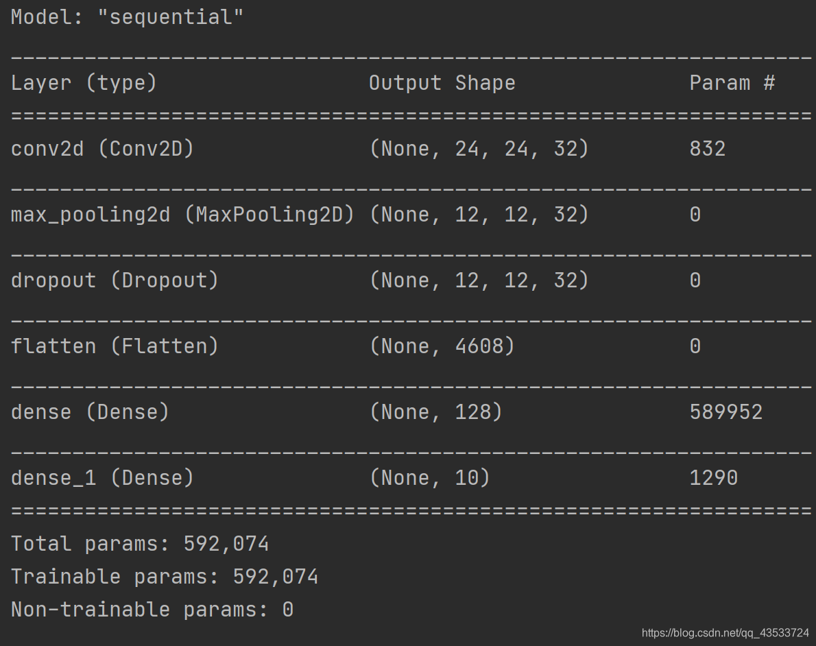
查看模型：

# 查看模型
model.summary()
for layer in model.layers:
    print(layer.get_output_at(0).get_shape().as_list())

在这里插入图片描述

训练模型：

# 训练模型，保存到history中
history =model.fit(train_X,train_Y,epochs=10,batch_size=200,verbose=2,validation_data=(test_X, test_Y))
# verbose=2  仅输出每个epoch的最终结果

绘制折线图：

fig = plt.figure()
plt.subplot(2, 1, 1)
plt.plot(history.history['accuracy'])
plt.plot(history.history['val_accuracy'])
plt.title('Model Accuracy')
plt.ylabel('accuracy')
plt.xlabel('epoch')
plt.legend(['train', 'test'], loc='lower right')

plt.subplot(2, 1, 2)
plt.plot(history.history['loss'])
plt.plot(history.history['val_loss'])
plt.title('Model Loss')
plt.ylabel('loss')
plt.xlabel('epoch')
plt.legend(['train', 'test'], loc='upper right')
plt.tight_layout()

plt.show()

保存模型：

# 保存模型
gfile = tf.io.gfile
save_dir = "./MNIST_model/"
if gfile.exists(save_dir):
    gfile.rmtree(save_dir)
gfile.mkdir(save_dir)

model_name = 'keras_mnist.h5'
model_path = os.path.join(save_dir, model_name)
model.save(model_path)
print('Saved trained model at %s ' % model_path)

加载模型并检测正确率：

# 加载模型
mnist_model = tf.keras.models.load_model(model_path)

# 统计模型在测试上的分类结果
loss_and_metrics = mnist_model.evaluate(test_X, test_Y, verbose=2)

print("Test Loss: {}".format(loss_and_metrics[0]))
print("Test Accuracy: {}".format(loss_and_metrics[1] * 100))

在这里插入图片描述

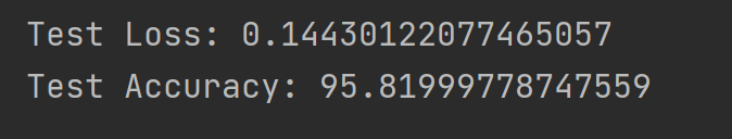
模型训练结果为95.81%，结果还没有MLP好，没事，我们还有更复杂的卷积神经网络。

完整代码：

import tensorflow as tf
from tensorflow.examples.tutorials.mnist import input_data
import matplotlib.pyplot as plt
import numpy as np
from keras.utils import np_utils
from keras.models import Sequential
from keras.layers import Dense
from keras.layers import Activation
from keras.layers import Conv2D
from keras.layers import Flatten
from keras.layers import MaxPooling2D
from keras.layers import Dropout
import os


mnist = input_data.read_data_sets('D:\pythonProject1\MNIST\MNIST_data',one_hot=True) # 热编码
train_X = mnist.train.images
train_Y = mnist.train.labels
test_X = mnist.test.images
test_Y = mnist.test.labels

print(train_X.shape, type(train_X))
print(test_X.shape, type(test_X))


train_X = train_X.reshape(train_X.shape[0],28,28,1)
test_X = test_X.reshape(test_X.shape[0],28,28,1)
print(train_X.shape, type(train_X)) # (55000,  28, 28,1 ) <class 'numpy.ndarray'>
print(test_X.shape, type(test_X)) # (10000,  28, 28, 1 ) <class 'numpy.ndarray'>

#数据归一化 min-max 标准化
train_X /= 255
test_X /= 255

def create_model():
    model = Sequential()
    model.add(Conv2D(filters=32, kernel_size=(5, 5), activation='relu',
                     input_shape=(28, 28, 1)))
    # 最大池化层，池化窗口 2x2
    model.add(MaxPooling2D(pool_size=(2, 2)))
    # Dropout 25% 的输入神经元
    model.add(Dropout(0.2))
    # 将 Pooled feature map 摊平后输入全连接网络
    model.add(Flatten())
    # 全联接层
    model.add(Dense(128, activation='relu'))
    # 使用 softmax 激活函数做多分类，输出各数字的概率
    model.add(Dense(10, activation='softmax'))
    # 编译模型
    model.compile(loss='categorical_crossentropy', metrics=['accuracy'], optimizer='adam')

    return model

model = create_model()

# 查看模型
model.summary()
for layer in model.layers:
    print(layer.get_output_at(0).get_shape().as_list())

# 训练模型，保存到history中
history =model.fit(train_X,train_Y,epochs=10,batch_size=200,verbose=2,validation_data=(test_X, test_Y))
# verbose=2  仅输出每个epoch的最终结果

# 可视化数据
fig = plt.figure()
plt.subplot(2, 1, 1)
plt.plot(history.history['accuracy'])
plt.plot(history.history['val_accuracy'])
plt.title('Model Accuracy')
plt.ylabel('accuracy')
plt.xlabel('epoch')
plt.legend(['train', 'test'], loc='lower right')

plt.subplot(2, 1, 2)
plt.plot(history.history['loss'])
plt.plot(history.history['val_loss'])
plt.title('Model Loss')
plt.ylabel('loss')
plt.xlabel('epoch')
plt.legend(['train', 'test'], loc='upper right')
plt.tight_layout()

plt.show()

# 保存模型
gfile = tf.io.gfile
save_dir = "./MNIST_model/"
if gfile.exists(save_dir):
    gfile.rmtree(save_dir)
gfile.mkdir(save_dir)

model_name = 'keras_mnist.h5'
model_path = os.path.join(save_dir, model_name)
model.save(model_path)
print('Saved trained model at %s ' % model_path)


# 加载模型
mnist_model = tf.keras.models.load_model(model_path)

# 统计模型在测试上的分类结果
loss_and_metrics = mnist_model.evaluate(test_X, test_Y, verbose=2)

print("Test Loss: {}".format(loss_and_metrics[0]))
print("Test Accuracy: {}".format(loss_and_metrics[1] * 100))