


卡尔曼预测在视觉跟踪中的运用
本文以byteTrack为例 进行分析
-
卡尔曼的五个公式
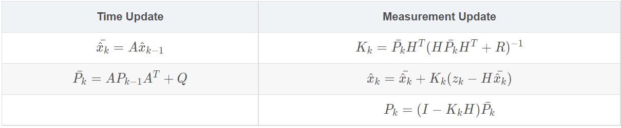
- 其中A 为状态转移矩阵
- P为协方差矩阵
- K为卡尔曼增益
- H为观测矩阵
-
在byteTrack中的代码实现过程:
-
其中卡尔曼的实现在项目的
 文件中
文件中 -
在视觉的目标跟踪一般是状态变量X采用(x, y, a, h, vx, vy, va, vh)观测变量Z采用(x, y, a, h)
- 状态变量X分别代表检测框的中心点:x,y 检测框的长宽比率a,以及检测框的高h,剩下的4个表示变换速率
- 观测变量Z分别代表检测框的中心点:x,y 检测框的长宽比率a,以及检测框的高h
- (在不太的跟踪器下 可能后面的a,h 选择使用S面积,以及高度h)
- (注意:只要状态变量能够完整描述整个系统即可)
-
主要是有一个卡尔曼类:
-
解析其中的代码
-
在__init__函数中:
-
def __init__(self): ndim, dt = 4, 1. # Create Kalman filter model matrices. self._motion_mat = np.eye(2 * ndim, 2 * ndim) for i in range(ndim): self._motion_mat[i, ndim + i] = dt # _motion_mat = [[1, 0, 0, 0, dt, 0, 0, 0], # [0, 1, 0, 0, 0, dt, 0, 0], # [0, 0, 1, 0, 0, 0, dt, 0], # [0, 0, 0, 1, 0, 0, 0, dt], # [0, 0, 0, 0, 1, 0, 0, 0], # [0, 0, 0, 0, 0, 1, 0, 0], # [0, 0, 0, 0, 0, 0, 1, 0], # [0, 0, 0, 0, 0, 0, 0, 1], # ] A矩阵 卡尔曼中的运动转移矩阵 self._update_mat = np.eye(ndim, 2 * ndim) # _update_mat = [[1, 0, 0, 0, 0, 0, 0, 0], # [0, 1, 0, 0, 0, 0, 0, 0], # [0, 0, 1, 0, 0, 0, 0, 0], # [0, 0, 0, 1, 0, 0, 0, 0], # ] H 矩阵 卡尔曼中的 观测矩阵 # Motion and observation uncertainty are chosen relative to the current # state estimate. These weights control the amount of uncertainty in # the model. This is a bit hacky. self._std_weight_position = 1. / 20 self._std_weight_velocity = 1. / 160 -
其中self._motion_mat中存的为卡尔曼中的A矩阵,其具体值为上文现实的样子(为什么是这样,是因为建模就是这样建立的,建立了一个恒定速度的模型)
-
其中self._update_mat是卡尔曼中的观测矩阵,这个很好理解 Z=HX(这是矩阵乘法,不可以随意调换顺序)
-
其中,self._std_weight_position,self._std_weight_velocity是Q、R调整参数 我们可以在后面看到
-
-
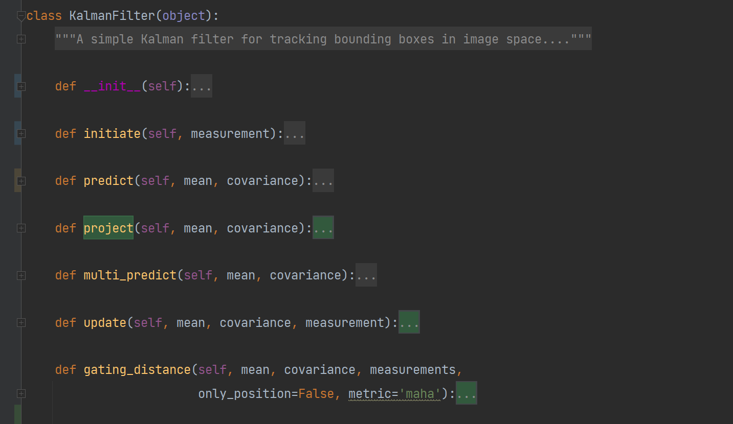
def project(self, mean, covariance):函数
-
def project(self, mean, covariance): """Project state distribution to measurement space. Parameters ---------- mean : ndarray The state's mean vector (8 dimensional array). covariance : ndarray The state's covariance matrix (8x8 dimensional). Returns ------- (ndarray, ndarray) Returns the projected mean and covariance matrix of the given state estimate. """ std = [ self._std_weight_position * mean[3], self._std_weight_position * mean[3], 1e-1, self._std_weight_position * mean[3]] innovation_cov = np.diag(np.square(std)) mean = np.dot(self._update_mat, mean) covariance = np.linalg.multi_dot(( self._update_mat, covariance, self._update_mat.T)) return mean, covariance + innovation_cov- 其中mean = HX
- 其中 innovation_cov为R 测量噪声协方差。滤波器实际实现时,测量噪声协方差 R一般可以观测得到,是滤波器的已知条件。
- 其中 covariance = H P H T HPH^T HPHT 为卡尔曼中[外链图片转存失败,源站可能有防盗链机制,建议将图片保存下来直接上传(img-jBS6e54W-1653305102843)(https://raw.githubusercontent.com/xifen523/img_typora_lib/main/img202205231652554.png)]
-
-
def initiate(self, measurement)函数:
-
初始化均值以及方差(就是卡尔曼中的X,以及P)
-
def initiate(self, measurement): """Create track from unassociated measurement. Parameters ---------- measurement : ndarray Bounding box coordinates (x, y, a, h) with center position (x, y), aspect ratio a, and height h. Returns ------- (ndarray, ndarray) Returns the mean vector (8 dimensional) and covariance matrix (8x8 dimensional) of the new track. Unobserved velocities are initialized to 0 mean. """ mean_pos = measurement mean_vel = np.zeros_like(mean_pos) mean = np.r_[mean_pos, mean_vel] # 按照列叠加 # mean = [ measurement[0], # measurement[1], # measurement[2], # measurement[3], # 0, # 0, # 0, # 0, # # ] X 状态向量 std = [ 2 * self._std_weight_position * measurement[3], 2 * self._std_weight_position * measurement[3], 1e-2, 2 * self._std_weight_position * measurement[3], 10 * self._std_weight_velocity * measurement[3], 10 * self._std_weight_velocity * measurement[3], 1e-5, 10 * self._std_weight_velocity * measurement[3]] covariance = np.diag(np.square(std)) # covariance = [[(2 * self._std_weight_position * measurement[3]) ** 2, 0, 0, 0, 0, 0, 0, 0], # [0, (2 * self._std_weight_position * measurement[3]) ** 2, 0, 0, 0, 0, 0, 0], # [0, 0, 1e-4, 0, 0, 0, 0, 0], # [0, 0, 0, (2 * self._std_weight_position * measurement[3]) ** 2, 0, 0, 0, 0], # [0, 0, 0, 0, (10 * self._std_weight_velocity * measurement[3]) ** 2, 0, 0, 0], # [0, 0, 0, 0, 0, (10 * self._std_weight_velocity * measurement[3]) ** 2, 0, 0], # [0, 0, 0, 0, 0, 0, 1e-5, 0], # [0, 0, 0, 0, 0, 0, 0, (10 * self._std_weight_velocity * measurement[3]) ** 2], # ] 初始化P矩阵 只要不是0矩阵就可以 return mean, covariance -
返回一个X,一个P
-
(其实只要维度对上就行了,X值随意,P只要不是0就行)
-
-
def predict(self, mean, covariance):函数
-
def predict(self, mean, covariance): """Run Kalman filter prediction step. Parameters ---------- mean : ndarray The 8 dimensional mean vector of the object state at the previous time step. covariance : ndarray The 8x8 dimensional covariance matrix of the object state at the previous time step. Returns ------- (ndarray, ndarray) Returns the mean vector and covariance matrix of the predicted state. Unobserved velocities are initialized to 0 mean. """ std_pos = [ self._std_weight_position * mean[3], self._std_weight_position * mean[3], 1e-2, self._std_weight_position * mean[3]] std_vel = [ self._std_weight_velocity * mean[3], self._std_weight_velocity * mean[3], 1e-5, self._std_weight_velocity * mean[3]] motion_cov = np.diag(np.square(np.r_[std_pos, std_vel])) # mean = np.dot(self._motion_mat, mean) mean = np.dot(mean, self._motion_mat.T) covariance = np.linalg.multi_dot(( self._motion_mat, covariance, self._motion_mat.T)) + motion_cov return mean, covariance -
其中
mean = np.dot(mean, self._motion_mat.T)对应卡尔曼中预测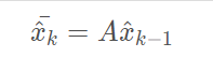
-
covariance = np.linalg.multi_dot((self._motion_mat, covariance, self._motion_mat.T)) + motion_cov对应
-
所以
motion_cov是卡尔曼中的Q矩阵,该参数被用来表示状态转换矩阵与实际过程之间的误差。因为我们无法直接观测到过程信号, 所以 Q 的取值是很难确定的。是卡尔曼滤波器用于估计离散时间过程的状态变量,也叫预测模型本身带来的噪声。
-
-
def update(self, mean, covariance, measurement):函数
-
def update(self, mean, covariance, measurement): """Run Kalman filter correction step. Parameters ---------- mean : ndarray The predicted state's mean vector (8 dimensional). covariance : ndarray The state's covariance matrix (8x8 dimensional). measurement : ndarray The 4 dimensional measurement vector (x, y, a, h), where (x, y) is the center position, a the aspect ratio, and h the height of the bounding box. Returns ------- (ndarray, ndarray) Returns the measurement-corrected state distribution. """ projected_mean, projected_cov = self.project(mean, covariance) chol_factor, lower = scipy.linalg.cho_factor( projected_cov, lower=True, check_finite=False) kalman_gain = scipy.linalg.cho_solve( (chol_factor, lower), np.dot(covariance, self._update_mat.T).T, check_finite=False).T innovation = measurement - projected_mean # z-HX new_mean = mean + np.dot(innovation, kalman_gain.T) # x+K(z-HX) new_covariance = covariance - np.linalg.multi_dot(( kalman_gain, projected_cov, kalman_gain.T)) return new_mean, new_covariance -
其中 projected_cov= H P H T + R HPH^T+R HPHT+R为卡尔曼中
-
projected_mean = HZ
-
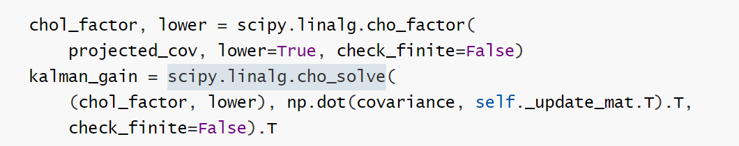
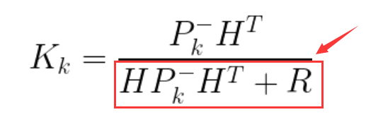
- 该部分为卡尔曼增益求解
- K k ( H P k − H T + R ) = P K − H T K_k(HP^-_kH^T+R)=P^-_KH^T Kk(HPk−HT+R)=PK−HT 其中 ( H P k − H T + R ) (HP^-_kH^T+R) (HPk−HT+R)的值就是projected_cov (定义为S的话)
- 将projected_cov 用scipy.linalg.cho_factor()分解
- 再用scipy.linalg.cho_solve()求解出 K k K_k Kk
-
new_covariance = covariance - np.linalg.multi_dot(( kalman_gain, projected_cov, kalman_gain.T))为卡尔曼中的: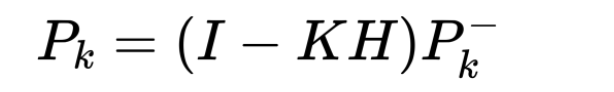
-
这个地方好像有点不一样 最后的P更新:
P k = P k − − ( K k ( H P k − H T + R ) K k T ) P_k=P^-_k-(K_k(HP^-_kH^T+R)K^T_k) Pk=Pk−−(Kk(HPk−HT+R)KkT) 这个怎么化简呢? 由前面可知: K k ( H P k − H T + R ) = P K − H T K_k(HP^-_kH^T+R)=P^-_KH^T Kk(HPk−HT+R)=PK−HT
则: P k = P k − − ( P K − H T ) K k T P_k=P^-_k-(P^-_KH^T)K^T_k Pk=Pk−−(PK−HT)KkT
-
这个地方化简不下去了 但是 计算的维度是对的 H是4X8 P是8X8 K是8X4
-
-
参考
- https://zhuanlan.zhihu.com/p/490226899
- https://zhuanlan.zhihu.com/p/36745755
- https://blog.youkuaiyun.com/lmm6895071/article/details/79771606?ops_request_misc=%257B%2522request%255Fid%2522%253A%2522165328039816782248588299%2522%252C%2522scm%2522%253A%252220140713.130102334.pc%255Fall.%2522%257D&request_id=165328039816782248588299&biz_id=0&utm_medium=distribute.pc_search_result.none-task-blog-2allfirst_rank_ecpm_v1~rank_v31_ecpm-2-79771606-null-null.142v10pc_search_result_control_group,157v4control&utm_term=%E4%B8%A4%E4%B8%AA%E9%AB%98%E6%96%AF%E5%88%86%E5%B8%83%E7%9A%84%E4%B9%98%E7%A7%AF+%E6%9C%89%E4%BB%80%E4%B9%88+%E6%84%8F%E4%B9%89&spm=1018.2226.3001.4187
- https://blog.youkuaiyun.com/u012912039/article/details/100771130?spm=1001.2101.3001.6650.4&utm_medium=distribute.pc_relevant.none-task-blog-2%7Edefault%7ECTRLIST%7ERate-4-100771130-blog-88697520.pc_relevant_antiscanv3&depth_1-utm_source=distribute.pc_relevant.none-task-blog-2%7Edefault%7ECTRLIST%7ERate-4-100771130-blog-88697520.pc_relevant_antiscanv3&utm_relevant_index=9


 5658
5658

 被折叠的 条评论
为什么被折叠?
被折叠的 条评论
为什么被折叠?
 到【灌水乐园】发言


