


用R做GLM的Summary相关指标解释
Residual
In ordinary least-squares, the residual associated with the i i i-th observation. The term residual comes from the residual sum of squares (RSS), which is defined as
r i = y i − f ( x i ) R S S = ∑ i = 1 n r i 2 r_i = y_i - f(x_i)\\ RSS=\sum_{i=1}^n r_i^2 ri=yi−f(xi)RSS=i=1∑nri2
where the residual r i r_i ri is defined as the difference between predicted values f ( x i ) f(x_i) f(xi) from the observed value y i y_i yi.
For GLMs, there are several ways for specifying residuals. We will cover four types of residuals: response residuals, working residuals, Pearson residuals, and, deviance residuals.
Response residuals
For type = "response", the conventional residual on the response level is computed, that is,
r
i
=
y
i
−
f
^
(
x
i
)
r_i=y_i−\hat f(x_i)
ri=yi−f^(xi)
# type = "response"
res.response1 <- residuals(model.pois, type = "response")
res.response2 <- expected - estimates
all.equal(res.response1, res.response2)
## [1] TRUE
Working residuals
For type = "working", the residuals are normalized by the estimates
f
^
(
x
i
)
\hat f(x_i)
f^(xi):
r i = y i − f ^ ( x i ) f ^ ( x i ) r_i=\frac{y_i−\hat f(x_i)}{\hat f(x_i)} ri=f^(xi)yi−f^(xi)
# type = "working"
res.working1 <- residuals(model.pois, type="working")
res.working2 <- (expected - estimates) / estimates
all.equal(res.working1, res.working2)
## [1] TRUE
Pearson residuals
For type = "pearson", the Pearson residuals are computed. They are obtained by normalizing the residuals by the square root of the estimate:
r i = y i − f ^ ( x i ) f ( x i ) r_i=\frac{y_i−\hat f(x_i)}{\sqrt{f(x_i)}} ri=f(xi)yi−f^(xi)
# type = "pearson"
res.pearson1 <- residuals(model.pois, type="pearson")
res.pearson2 <- (expected - estimates) / sqrt(estimates)
all.equal(res.pearson1, res.pearson2)
## [1] TRUE
Deviance residuals
Deviance residuals are defined by the deviance.
Deviance
The deviance of a model is given by
D ( y , μ ^ ) = 2 ( log ( p ( y ∣ θ ^ s ) ) − log ( p ( y ∣ θ ^ 0 ) ) ) D(y,\hat μ)=2(\log (p(y∣\hat θ_s))−\log (p(y∣\hat θ_0))) D(y,μ^)=2(log(p(y∣θ^s))−log(p(y∣θ^0)))
where
- y y y is the outcome.
- μ ^ \hat μ μ^ is the estimate of the model.
- θ ^ s \hat θ_s θ^s and θ ^ 0 \hat θ_0 θ^0 are the parameters of the fitted saturated and proposed models, respectively. A saturated model has as many parameters as it has training points, that is, p = n p=n p=n. Thus, it has a perfect fit. The proposed model can be the any other model.
- p(y|θ) is the likelihood of data given the model.
The deviance indicates the extent to which the likelihood of the saturated model exceeds the likelihood of the proposed model. If the proposed model has a good fit, the deviance will be small. If the proposed model has a bad fit, the deviance will be high. For example, for the Poisson model, the deviance is
D
=
2
⋅
∑
i
=
1
n
[
y
i
⋅
log
(
y
i
μ
^
i
)
−
(
y
i
−
μ
^
i
)
]
D=2 \cdot \sum_{i=1}^n \left[ y_i \cdot \log (\frac{y_i}{\hat μ_i})−(y_i−\hat μ_i) \right]
D=2⋅i=1∑n[yi⋅log(μ^iyi)−(yi−μ^i)]
具体推导过程参考: Poission regression deviance 的推导
-
首先假设 x x x只有一个位置参数, Y Y Y 服从Poission distribution,并且 Y Y Y 的均值是一个关于 x x x 的函数,即
E ( Y ∣ x ) = λ ( x ) \mathbb E(Y|x) = \lambda (x) E(Y∣x)=λ(x) -
对于Poission regression用 log \log log 作为link function,即 log ( λ ( x ) ) = β 0 + β 1 x \log(\lambda(x))=\beta_0 + \beta_1 x log(λ(x))=β0+β1x
-
那么Likelihood function就是 L ( β 0 , β 1 ; y i ) = ∏ i = 1 n e − λ ( x i ) [ λ ( x i ) y i ] y i ! = ∏ i = 1 n e e − β 0 + β 1 x i [ e β 0 + β 1 x i ] y i ] y i ! L(\beta_0, \beta_1; y_i) = \prod \limits_{i=1}^n \frac{e^{-\lambda(x_i)}[\lambda(x_i)^{y_i}]}{y_i !} = \prod \limits_{i=1}^n \frac{e^{e^{-\beta_0 + \beta_1 x_i}}[e^{\beta_0 + \beta_1 x_i}]^{y_i}]}{y_i !} L(β0,β1;yi)=i=1∏nyi!e−λ(xi)[λ(xi)yi]=i=1∏nyi!ee−β0+β1xi[eβ0+β1xi]yi]
Log likelihood function就是:
l
(
β
0
,
β
1
;
y
i
)
=
∑
i
=
1
n
y
i
(
β
0
+
β
1
x
i
)
−
∑
i
=
1
n
e
β
0
+
β
1
x
i
−
∑
i
=
1
n
log
(
y
i
!
)
(
1
)
l(\beta_0, \beta_1; y_i) = \sum \limits_{i=1}^n y_i(\beta_0 + \beta_1 x_i) - \sum \limits_{i=1}^n e^{\beta_0 + \beta_1 x_i} - \sum \limits_{i=1}^n \log (y_i !) \quad \quad (1)
l(β0,β1;yi)=i=1∑nyi(β0+β1xi)−i=1∑neβ0+β1xi−i=1∑nlog(yi!)(1)
写成用
μ
^
i
\hat \mu_i
μ^i表示均值预测值的形式,即
l
(
μ
^
)
=
∑
i
=
1
n
y
i
log
(
μ
^
i
)
−
∑
i
=
1
n
μ
^
i
−
∑
i
=
1
n
log
(
y
i
!
)
(
1
′
)
l(\hat \mu) = \sum \limits_{i=1}^n y_i \log(\hat \mu_i) - \sum \limits_{i=1}^n {\hat \mu_i} - \sum \limits_{i=1}^n \log (y_i !) \quad \quad (1')
l(μ^)=i=1∑nyilog(μ^i)−i=1∑nμ^i−i=1∑nlog(yi!)(1′)
- 用 μ 1 , μ 2 , ⋯ , μ n \mu_1,\mu_2,\cdots,\mu_n μ1,μ2,⋯,μn代替"saturated model"的参数(saturated model:每个数据点都有一个自己的参数构成的模型)。
那么,saturated model 的 log likelihood function 即为:
l
(
μ
)
=
∑
i
=
1
n
y
i
log
(
μ
i
)
−
∑
i
=
1
n
μ
i
−
∑
i
=
1
n
log
(
y
i
!
)
(
2
)
l(\mu) = \sum \limits_{i=1}^n y_i \log(\mu_i) - \sum \limits_{i=1}^n {\mu_i} - \sum \limits_{i=1}^n \log (y_i !) \quad \quad (2)
l(μ)=i=1∑nyilog(μi)−i=1∑nμi−i=1∑nlog(yi!)(2)
欲求(2)式中
μ
i
\mu_i
μi的最优估计,即对(2)求偏导数,并令其等于0,即:
∂
∂
μ
i
l
(
μ
)
=
y
i
μ
i
−
1
=
0
\frac{\partial}{\partial \mu_i}l(\mu) = \frac{y_i}{\mu_i} - 1=0
∂μi∂l(μ)=μiyi−1=0
解得,’‘saturated model’’ 的参数估计值为:
μ
^
i
=
y
i
\hat \mu_i = y_i
μ^i=yi
将上面的结果带入到(2)式中,即得“saturated model”的likelihood function:
l
(
μ
^
)
=
∑
i
=
1
n
y
i
log
(
y
i
)
−
∑
i
=
1
n
y
i
−
∑
i
=
1
n
log
(
y
i
!
)
(
3
)
l(\hat \mu) = \sum \limits_{i=1}^n y_i \log(y_i) - \sum \limits_{i=1}^n {y_i} - \sum \limits_{i=1}^n \log (y_i !) \quad \quad (3)
l(μ^)=i=1∑nyilog(yi)−i=1∑nyi−i=1∑nlog(yi!)(3)
- 由Deviance的定义:
D
(
y
,
μ
^
)
=
2
(
log
(
p
(
y
∣
θ
^
s
)
)
−
log
(
p
(
y
∣
θ
^
0
)
)
)
D(y,\hat μ)=2(\log (p(y∣\hat θ_s))−\log (p(y∣\hat θ_0)))
D(y,μ^)=2(log(p(y∣θ^s))−log(p(y∣θ^0))),即用
2
⋅
[
(
3
)
−
(
1
′
)
]
,
得
2 \cdot [(3)-(1')],得
2⋅[(3)−(1′)],得:
D ( y , μ ^ ) = 2 ⋅ [ ∑ i = 1 n y i log y i μ ^ i − ∑ i = 1 n ( y i − μ ^ i ) ] D(y,\hat \mu)=2 \cdot \left[\sum \limits_{i=1}^n y_i \log \frac{y_i}{\hat \mu_i} - \sum \limits_{i=1}^n (y_i - \hat \mu_i) \right] D(y,μ^)=2⋅[i=1∑nyilogμ^iyi−i=1∑n(yi−μ^i)]
注意:这仅仅对于分类模型,有时也用 (D)表示Deviance, (D∗)表示Scaled Deviance,即D除以上一个尺度参数。
即
D
∗
=
D
⋅
ϕ
D^{*}=D \cdot \phi
D∗=D⋅ϕ
例如,Poission分布的尺度参数就为1,Nomal distribution的尺度参数为
σ
2
\sigma^2
σ2.
所以,Nomal distribution的Deviance推出来是
D
(
y
,
μ
)
=
(
y
−
μ
)
2
D(y,\mu)=(y−\mu)^2
D(y,μ)=(y−μ)2
Scaled Deviance是
D
∗
(
y
,
μ
)
=
(
y
−
μ
)
2
σ
2
D^{*}(y,\mu)=\frac{(y−\mu)^2}{\sigma^2}
D∗(y,μ)=σ2(y−μ)2
详情https://stats.stackexchange.com/questions/315788/deviance-in-simple-linear-regression
Deviance residuals
In R, the deviance residuals represent the contributions of individual samples to the deviance D. More specifically, they are defined as the signed square roots of the unit deviances.
How does such a deviance look like in practice? For example, for the Poisson distribution, the deviance residuals are defined as:(这里我个人有个小疑问暂时没解决,根号下的数不一定是正的呀)
r i = s i g n ( y − μ ^ i ) ⋅ 2 ⋅ [ y i ⋅ log ( y i μ ^ i ) − ( y i − μ ^ i ) ] r_i=sign (y−\hat μ_i) \cdot \sqrt{2 \cdot \left[ y_i⋅\log \left( \frac{y_i} {\hat μ_i} \right)−(y_i−\hat μ_i) \right]} ri=sign(y−μ^i)⋅2⋅[yi⋅log(μ^iyi)−(yi−μ^i)]
# type = "deviance"
res.dev1 <- residuals(model.pois, type = "deviance")
res.dev2 <- residuals(model.pois)
poisson.dev <- function (y, mu)
    # unit deviance
    2 * (y * log(ifelse(y == 0, 1, y/mu)) - (y - mu))
res.dev3 <- sqrt(poisson.dev(expected, estimates)) *
        ifelse(expected > estimates, 1, -1)
all.equal(res.dev1, res.dev2, res.dev3)
## [1] TRUE
Deviance residuals举例
We can obtain the deviance residuals of our model using the residuals function:
summary(residuals(model.pois))
如果有以下输出
##    Min. 1st Qu.  Median    Mean 3rd Qu.    Max.
## -4.0451 -2.4138 -0.8169 -0.1840  1.4265  8.7946
Since the median deviance residual is close to zero, this means that our model is not biased in one direction (i.e. the out come is neither over- nor underestimated).
Tips:
Note that, for ordinary least-squares models, the deviance residual is identical to the conventional residual.
推导见:
https://bookdown.org/egarpor/PM-UC3M/glm-deviance.html#eq:dev
或者
https://stats.stackexchange.com/questions/315788/deviance-in-simple-linear-regression
Residual 小结
| 名称 | Response residuals(conventional residuals) | Working residuals | Pearson residuals | Deviance residuals |
|---|---|---|---|---|
| 公式 | r i = y i − f ^ ( x i ) r_i=y_i−\hat f(x_i) ri=yi−f^(xi) | r i = y i − f ^ ( x i ) f ^ ( x i ) r_i=\frac{y_i−\hat f(x_i)}{\hat f(x_i)} ri=f^(xi)yi−f^(xi) | r i = y i − f ^ ( x i ) f ( x i ) r_i=\frac{y_i−\hat f(x_i)}{\sqrt{f(x_i)}} ri=f(xi)yi−f^(xi) | r i = s i g n ( y − μ ^ i ) ⋅ 2 ⋅ [ y i ⋅ log ( y i μ ^ i ) − ( y i − μ ^ i ) ] r_i=sign (y−\hat μ_i) \cdot \sqrt{2 \cdot \left[ y_i⋅\log \left( \frac{y_i} {\hat μ_i} \right)−(y_i−\hat μ_i) \right]} ri=sign(y−μ^i)⋅2⋅[yi⋅log(μ^iyi)−(yi−μ^i)] |
| 意义 | 常规 | Normalize by the estimates | Normalize the residuals by the square root of the estimate | represent the contributions of individual samples to the deviance D D D |
Null Deviance and Residual Deviance
图解Null model, proposed model and saturated model——以Nomal regression为例
这部分参考了视频:https://www.youtube.com/watch?v=9T0wlKdew6I&t=0s
我们假设只有均值这一种未知参数(即方差已知)。
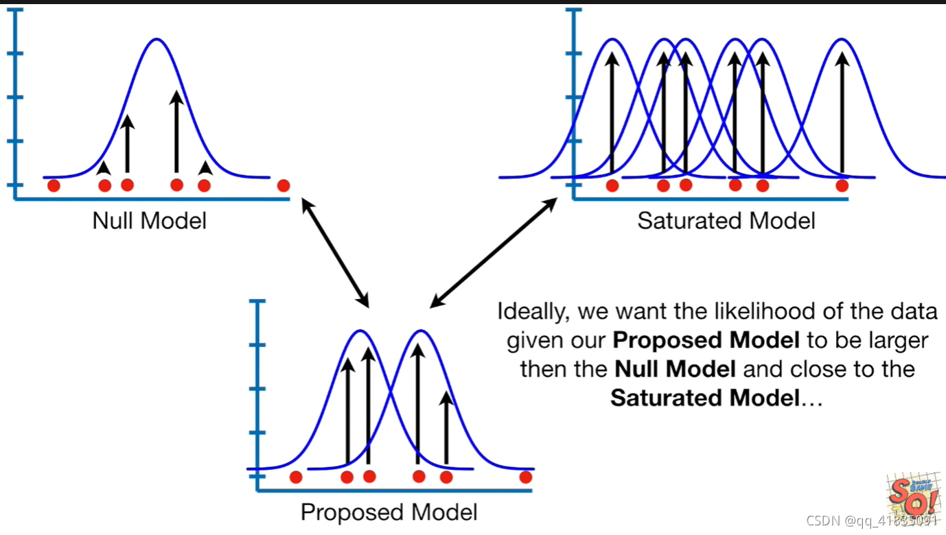
如图,左上角的就是Null model,即这些数据只用一个参数去刻画;右上角的就是Saturated Model,即每个数据都有一个参数刻画它,模型很饱和;下方的是Proposed Model,即我们使用的模型,需要去评估的模型,它可以是任何介于Null Model和Saturated Model之间的模型。
Since we have already introduced the deviance, understanding the null and residual deviance is not a challenge anymore. Let us repeat the definition of the deviance once again:
D ( y , μ ) = 2 ( log ( p ( y ∣ θ s ) ) − log ( p ( y ∣ θ 0 ) ) ) D(y,\mu)=2(\log(p(y∣\theta^s))−\log(p(y∣\theta^0))) D(y,μ)=2(log(p(y∣θs))−log(p(y∣θ0)))
The null and residual deviance differ in θ 0 θ_0 θ0:
- Null deviance: θ 0 θ_0 θ0 refers to the null model (i.e. an intercept-only model)
- Residual deviance: θ 0 θ_0 θ0 refers to the trained model
How can we interpret these two quantities?
- Null deviance: A low null deviance implies that the data can be modeled well merely using the intercept. If the null deviance is low, you should consider using few features for modeling the data.
- Residual deviance: A low residual deviance implies that the model you have trained is appropriate. Congratulations!
图解:

Confusing one: Deviance Residuals VS Residual Deviance
| 名称 | Deviance Residuals | Residual Deviance |
|---|---|---|
| 公式 | r i = s i g n ( y − μ ^ i ) ⋅ 2 ⋅ [ y i ⋅ log ( y i μ ^ i ) − ( y i − μ ^ i ) ] r_i=sign (y−\hat μ_i) \cdot \sqrt{2 \cdot \left[ y_i⋅\log \left( \frac{y_i} {\hat μ_i} \right)−(y_i−\hat μ_i) \right]} ri=sign(y−μ^i)⋅2⋅[yi⋅log(μ^iyi)−(yi−μ^i)] | R e s i d u a l D e v i a n c e = ∑ [ ( D e v i a n c e R e s i d u a l ) i ] 2 Residual Deviance =\sum[(Deviance \, \, Residual)_i]^2 ResidualDeviance=∑[(DevianceResidual)i]2 D ( y , μ ^ ) = 2 ( log ( p ( y ∣ θ ^ s ) ) − log ( p ( y ∣ θ ^ 0 ) ) ) D(y,\hat μ)=2(\log (p(y∣\hat θ_s))−\log (p(y∣\hat θ_0))) D(y,μ^)=2(log(p(y∣θ^s))−log(p(y∣θ^0))) |
| 区别 | Deviance Residuals是Residual的一种,重点关注每个样本点,区别于上文提到的另外三种Residual | Residual Deviance是Deviance的一种,重点关注模型整体,是‘saturated model’与‘proposed model’的log likelihood差的二倍,区别于Null Deviance( ‘saturated model’ 与 ‘null model’ 的log likelihood差的二倍) |
Other outputs of the summary function
Here, I deal with the other outputs of the GLM summary fuction: the dispersion parameter, the AIC, and the statement about Fisher scoring iterations.
Dispersion parameter
Dispersion (variability/scatter/spread) simply indicates whether a distribution is wide or narrow. The GLM function can use a dispersion parameter to model the variability.
However, for likelihood-based model, the dispersion parameter is always fixed to 1. It is adjusted only for methods that are based on quasi-likelihood estimation such as when family = "quasipoisson" or family = "quasibinomial". These methods are particularly suited for dealing with overdispersion.
AIC
The Akaike information criterion (AIC) is an information-theoretic measure that describes the quality of a model. It is defined as
A I C = 2 p − 2 ln ( L ^ ) AIC=2p−2 \ln (\hat L) AIC=2p−2ln(L^)
where p p p is the number of model parameters and L ^ \hat L L^ is the maximum of the likelihood function. A model with a low AIC is characterized by low complexity (minimizes p p p) and a good fit (maximizes L ^ \hat L L^).


 2630
2630

 被折叠的 条评论
为什么被折叠?
被折叠的 条评论
为什么被折叠?
 到【灌水乐园】发言


