scipy函数：scipy.optimize.fminbound 函数分析

为什么要做这个分析？

我试图用c语言翻译scipy.signal中的iirfilter函数，其中用到了fminbound。当使用我自定义的求极小值函数时，得到的传递函数系数值在小数点后四到五位有误差，但是得到的滤波器幅频响应差别很大，很不理想。强行翻译fminbound后无法正确输出。因此还是决定先理解，再编程。可把宝宝为难坏了。

scipy.optimize.fminbound官方说明
参考书：《C++数值算法》普雷斯著

scipy.optimize.fminbound

参数分析

def fminbound(func, x1, x2, args=(), xtol=1e-5, maxfun=500,
              full_output=0, disp=1):
              
    options = {'xatol': xtol,
               'maxiter': maxfun,
               'disp': disp}

    res = _minimize_scalar_bounded(func, (x1, x2), args, **options)
    if full_output:
        return res['x'], res['fun'], res['status'], res['nfev']
    else:
        return res['x']

Parameters

• func: callable f(x, *args)
  Objective function to be minimized (must accept and return scalars).
  欲取极小值的目标函数（必须接受并返回标量）

• x1, x2: float or array scalar
  The optimization bounds.
  取极小值的区间

• args: tuple, optional
  Extra arguments passed to functions.
  目标函数的其他输入参数

• xtop: float, optional
  The convergence tolerance.
  收敛容差，我理解是一个很小的常量

• maxfun: int, optional
  Maximum number of function evaluations allowed.
  最大循环次数，如果在此次数之间没有得到极小值则跳出循环

• full_output: bool, optional
  If true, return optional outputs.

• disp: int, optional
  If non-zero, print messages.
  0: no message printing.
  1: non-convergence notification messages only.
  2: print a message on convergence too.
  3: print iteration results.

Returns

• xopt: ndarray
  Parameters (over given interval) which minimize the objective function.
  res[‘x’] 输出极小值的x值

• fval: number
  The function value at the minimum point
  res[‘fun’] 极小值的y值

• ierr: int
  An error flag (0 if converged, 1 if maximum number of function calls reached).
  res[‘status’]

• numfunc: int
  The number of function calls made.
  res[‘nfev’]

_minimize_scalar_bounded

这个函数非常长，因此我决定分步进行。

def _minimize_scalar_bounded(func, bounds, args=(),
                             xatol=1e-5, maxiter=500, disp=0,
                             **unknown_options):

Parameters

• maxiter : int
  Maximum number of iterations to perform.
  最大迭代次数

• disp: int, optional
  If non-zero, print messages.
  0 : no message printing.
  1 : non-convergence notification messages only.
  2 : print a message on convergence too.
  3 : print iteration results.

• xatol : float
  Absolute error in solution xopt acceptable for convergence.

循环外

循环外定义以下参数：

常数

• xatol = 1e-5                # 收敛容差，为恰巧为0的极小值情况而设置的一个相对精确的小数
• maxfun = maxfun = 500          # 最大迭代次数
• sqrt_eps = sqrt(2.2e-16)         # eps的开方，机器浮点精度的平方根，返回值的相对精度
• golden_mean = 0.5 * (3.0 - sqrt(5.0))  # 黄金分割点

变量

储存x与y值的变量

•  fulc,  nfc, xf,  x  # 储存x
• ffulc, fnfc, fx, fu  # 储存y

其他变量

• a, b # 取值区间
• num # 迭代次数
• fmin_data = (1, x, y) # 储存当前迭代的次数以及x, y值
• flag = 0 # 状态判定
• xm = 0.5 * (a + b) # 当前范围的中点
• rat = e = 0.0 # 步长？
• tol1, tol2 # 判别值，其中tol1中唯一的变量为xf

循环内分析

Brent方法：x, y, a, b

		# 用某种方式更新x, fu
        x = xf + si * np.maximum(np.abs(rat), tol1)
        fu = func(x, *args)
        num += 1 # 更新迭代次数
        fmin_data = (num, x, fu) # 储存当前值
        if disp > 2:
            print("%5.0f   %12.6g %12.6g %s" % (fmin_data + (step,)))

		# 以下为x, y, a, b的更新
        if fu <= fx: 						# 条件 1
            if x >= xf: 					# 条件 1-1
                a = xf
            else:							# 条件 1-2
                b = xf
            fulc, ffulc = nfc, fnfc
            nfc, fnfc = xf, fx
            xf, fx = x, fu
        else:								# 条件 2
            if x < xf:						# 条件 2-1
                a = x
            else:							# 条件 2-2
                b = x
            if (fu <= fnfc) or (nfc == xf):							# 条件 2-1-1 或 2-2-1
                fulc, ffulc = nfc, fnfc
                nfc, fnfc = x, fu
            elif (fu <= ffulc) or (fulc == xf) or (fulc == nfc):	# 条件 2-1-2 或 2-2-2
                fulc, ffulc = x, fu

• 开始循环之前：

  • 设(x₀, y₀), [a₀, b₀]。有：
    代表x的值：
    fulc = nfc = xf = x = x₀
    代表y的值：
    ffulc = fnfc = fx = y₀
    fu = np.inf

• 第一次循环：

  • 生成新的(x, fu) → (x₁, y₁)
  • 更新：若满足条件 1-1:
    fu <= fx & x < xf 函数下降
    a₁ = xf = x₀, b₁ = b₀   (a₁, b₁) → (x₀, b₀)
    fulc, ffulc = nfc, fnfc   (fulc, ffulc) → (x₀, y₀)  对应位置a₁
    nfc, fnfc = xf, fx    (nfc, fnfc) → (x₀, y₀)   对应位置a₁
    xf, fx= x, fu        (fulc, ffulc) → (x₁, y₁)  对应位置为a₁b₁之间

• 第二次循环：

  • 生成新的(x, fu) → (x₂, y₂)
  • 更新：若满足条件 1-2:
    fu <= fx & x > xf 函数上升
    a₂ = a₁ = x₀, b₂ = xf = x₁ (a₁, b₁) → (x₀, x₁)
    fulc, ffulc = nfc, fnfc   (fulc, ffulc) → (x₀, y₀)  对应位置a₂
    nfc, fnfc = xf, fx    (nfc, fnfc) → (x₁, y₁)   对应位置b₂
    xf, fx= x, fu        (fulc, ffulc) → (x₂, y₂)  对应位置为a₂b₂之间

• 第三次循环：

  • 生成新的(x, fu) → (x₃, y₃)
  • 更新：若满足条件 2-1-1:
    fu > fx & x < xf 函数下降
    a₃ = x = x₃, b₃ = b₂ = x₁ (a₃, b₃) → (x₃, x₁)
    fu <= fnfc (y₃ <= y₁) or nfc == xf (x₁ == x₂)
    fulc, ffulc = nfc, fnfc   (fulc, ffulc) → (x₁, y₁)  对应位置b₃
    nfc, fnfc = x, fu     (nfc, fnfc) → (x₃, y₃)   对应位置a₃
    xf, fx          (fulc, ffulc) → (x₂, y₂)  对应位置为a₃b₃之间

• 第四次循环：

  • 生成新的(x, fu) → (x₄, y₄)
  • 更新：若满足条件 2-2-2:
    fu > fx & x 》= xf 函数上升
    a₄ = a₃ = x₃, b₄ = x = x₄ (a₃, b₃) → (x₃, x₄)
    fu <= ffulc (y₄ <= y₁) or fulc == xf (x₁ == x₂) or fulc == nfc (x₁ == x₃)
    fulc, ffulc = x, fu   (fulc, ffulc) → (x₄, y₄)  对应位置a₄
    nfc, fnfc        (nfc, fnfc) → (x₃, y₃)   对应位置b₄
    xf, fx          (fulc, ffulc) → (x₂, y₂)  对应位置为a₄b₄之间

• 小结：

  由以上过程可知：(fulc, ffulc)， (nfc, fnfc) 分别保存两个端点(a, b) 的函数值；(xf, fx) 保存两者之间的一个函数值，也可以说是目前最佳的迭代结果。而 fmin_data 却不如它名字那般是储存最小值，而是最新一次迭代的结果，在条件 2-x-x 中，它并不是最佳的迭代结果。fmin_data 在整个函数中唯一的作用是打印当前迭代结果，在翻译时可以忽略。

抛物线内插法：r, q, p

        if np.abs(e) > tol1:
            golden = 0
            r = (xf - nfc) * (fx - ffulc)
            q = (xf - fulc) * (fx - fnfc)
            p = (xf - fulc) * q - (xf - nfc) * r
            q = 2.0 * (q - r)
            if q > 0.0:
                p = -p
            q = np.abs(q)
            r = e
            e = rat

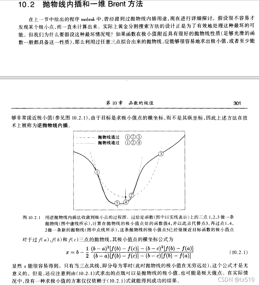
已知逆抛物线内插法公式：
对于过 $f(a)$， $f(b)$ 和 $f(c)$ 三点的抛物线，其极小值点的横坐标公式为
$$x=b-\frac{1}{2}\frac{(b-a{)}^2[f(b)-f(c)]-(b-c{)}^2[f(b)-f(a)]}{(b-a)[f(b)-f(c)]-(b-c)[f(b)-f(a)]}$$
，其中 $a<b<c$ 且 $f(b)<f(a)$， $f(b)<f(c)$。
利用这个公式来理解r, q, p。

设 (fulc, ffulc) = (a, f(a))
  (xf, fx)    = (b, f(b))
  (nfc, fnfc)  = (c, f(c ))
其中 a < b < c，f(b) < f(a)，f(b) < f(c )

r = (xf - nfc) * (fx - ffulc) # = (b - c) * [f(b) - f(a)]
q = (xf - fulc) * (fx - fnfc) # = (b - a) * [f(b) - f(c)]
p = (xf - fulc) * q - (xf - nfc) * r
	# = (b - a) * q - (b - c) * r
	# = (b - a) ** 2 * [f(b) - f(c)] - (b - c) ** 2 * [f(b) - f(a)]
	# 即内插公式的分子
q = 2.0 * (q - r) # 即内插公式的分母
if q > 0.0:
	p = -p
q = np.abs(q)
# 这三行等同于：
# if q > 0.0: p = -p, q = q
# else:       p = p, q = -q
# 这样保证 p / q 的结果前面为负号，而q非负

• 小结

  这一部分是构造一个试探用的抛物线拟合。整个算法的思路就是：当函数不配合抛物线拟合的时候，用另一种收敛速度缓慢但很可靠的技巧（比如黄金分割搜索方法，即Brent算法）来求解，而在目标函数允许的情况下，转而使用逆抛物线内插法求解。
  据此，下一个步骤为：判断抛物线内插是否合适。若合适，采用抛物线内插法；若不合适，在较长区间段采用黄金分割法。

判断是否使用抛物线内插法

            # Check for acceptability of parabola
            if ((np.abs(p) < np.abs(0.5*q*r)) and (p > q*(a - xf)) and
                    (p < q * (b - xf))):
                rat = (p + 0.0) / q
                x = xf + rat
                step = '       parabolic'

                if ((x - a) < tol2) or ((b - x) < tol2):
                    si = np.sign(xm - xf) + ((xm - xf) == 0)
                    rat = tol1 * si
            else:      # do a golden-section step
                golden = 1

已知q非负。分析if内条件：（设逆抛物线内插法所得横坐标为 x₀ ）

• $|p|<|0.5\times q\times r|$ 相当于 $\frac{|p|}{2q}<|r|$，即
  $$x_0=xf-\frac{p}{2q}\in [xf-|r|,xf+|r|]$$
• $p>q\times (a-xf)\cup p<q\times (b-xf)$ 相当于
  $$a-xf<\frac{p}{q}<b-xf$$
  即
  $$xf-\frac{b-xf}{2}<x_0<xf+\frac{xf-a}{2}$$

根据参考书所说：

为了达到求解目的，抛物线必须满足：(i) 在限定区域(a, b)内下降；(ii) 从当前最佳值x移动的步长能够小于前面第二步移动步长的一半。后一条准则保证了内插步骤可以有效地收敛到某点，而不会在某一非收敛的有限范围内跳跃。

判定结果即满足条件 (ii) 。如果判定为真，则进行逆抛物线内插法，否则进行黄金分割法。

python.scipy._minimize_scalar_bounded 源代码

def _minimize_scalar_bounded(func, bounds, args=(),
                             xatol=1e-5, maxiter=500, disp=0,
                             **unknown_options):
    """
    Options
    -------
    maxiter : int
        Maximum number of iterations to perform.
    disp: int, optional
        If non-zero, print messages.
            0 : no message printing.
            1 : non-convergence notification messages only.
            2 : print a message on convergence too.
            3 : print iteration results.
    xatol : float
        Absolute error in solution `xopt` acceptable for convergence.

    """
    _check_unknown_options(unknown_options)
    maxfun = maxiter
    # Test bounds are of correct form
    if len(bounds) != 2:
        raise ValueError('bounds must have two elements.')
    x1, x2 = bounds

    if not (is_array_scalar(x1) and is_array_scalar(x2)):
        raise ValueError("Optimization bounds must be scalars"
                         " or array scalars.")
    if x1 > x2:
        raise ValueError("The lower bound exceeds the upper bound.")

    flag = 0
    header = ' Func-count     x          f(x)          Procedure'
    step = '       initial'

    sqrt_eps = sqrt(2.2e-16)
    golden_mean = 0.5 * (3.0 - sqrt(5.0))
    a, b = x1, x2
    fulc = a + golden_mean * (b - a)
    nfc, xf = fulc, fulc
    rat = e = 0.0
    x = xf
    fx = func(x, *args)
    num = 1
    fmin_data = (1, xf, fx)
    fu = np.inf

    ffulc = fnfc = fx
    xm = 0.5 * (a + b)
    tol1 = sqrt_eps * np.abs(xf) + xatol / 3.0
    tol2 = 2.0 * tol1

    if disp > 2:
        print(" ")
        print(header)
        print("%5.0f   %12.6g %12.6g %s" % (fmin_data + (step,)))

    while (np.abs(xf - xm) > (tol2 - 0.5 * (b - a))):
        golden = 1
        # Check for parabolic fit
        if np.abs(e) > tol1:
            golden = 0
            r = (xf - nfc) * (fx - ffulc)
            q = (xf - fulc) * (fx - fnfc)
            p = (xf - fulc) * q - (xf - nfc) * r
            q = 2.0 * (q - r)
            if q > 0.0:
                p = -p
            q = np.abs(q)
            r = e
            e = rat

            # Check for acceptability of parabola
            if ((np.abs(p) < np.abs(0.5*q*r)) and (p > q*(a - xf)) and
                    (p < q * (b - xf))):
                rat = (p + 0.0) / q
                x = xf + rat
                step = '       parabolic'

                if ((x - a) < tol2) or ((b - x) < tol2):
                    si = np.sign(xm - xf) + ((xm - xf) == 0)
                    rat = tol1 * si
            else:      # do a golden-section step
                golden = 1

        if golden:  # do a golden-section step
            if xf >= xm:
                e = a - xf
            else:
                e = b - xf
            rat = golden_mean*e
            step = '       golden'

        si = np.sign(rat) + (rat == 0)
        x = xf + si * np.maximum(np.abs(rat), tol1)
        fu = func(x, *args)
        num += 1
        fmin_data = (num, x, fu)
        if disp > 2:
            print("%5.0f   %12.6g %12.6g %s" % (fmin_data + (step,)))

        if fu <= fx:
            if x >= xf:
                a = xf
            else:
                b = xf
            fulc, ffulc = nfc, fnfc
            nfc, fnfc = xf, fx
            xf, fx = x, fu
        else:
            if x < xf:
                a = x
            else:
                b = x
            if (fu <= fnfc) or (nfc == xf):
                fulc, ffulc = nfc, fnfc
                nfc, fnfc = x, fu
            elif (fu <= ffulc) or (fulc == xf) or (fulc == nfc):
                fulc, ffulc = x, fu

        xm = 0.5 * (a + b)
        tol1 = sqrt_eps * np.abs(xf) + xatol / 3.0
        tol2 = 2.0 * tol1

        if num >= maxfun:
            flag = 1
            break

    if np.isnan(xf) or np.isnan(fx) or np.isnan(fu):
        flag = 2

    fval = fx
    if disp > 0:
        _endprint(x, flag, fval, maxfun, xatol, disp)

    result = OptimizeResult(fun=fval, status=flag, success=(flag == 0),
                            message={0: 'Solution found.',
                                     1: 'Maximum number of function calls '
                                        'reached.',
                                     2: _status_message['nan']}.get(flag, ''),
                            x=xf, nfev=num)

    return result

翻译的c函数：(其中传递的函数指针只有一个double形参，如果函数还有其他形参，需要加上)

double sign(double x)
{
	return (x >= 0.) ? 1. : -1.;
}

double MinimizerBrent(double (*func)(double), double x1, double x2)
{
	double xatol, maxiter, sqrt_eps, golden_mean;
	xatol = 1e-5;
	maxiter = 500;
	sqrt_eps = sqrt(2.2e-16);
	golden_mean = 0.5 * (3. - sqrt(5.));

	int flag = 0;

	double a, b;
	a = x1;
	b = x2;
	
	// x
	double x, xf, fx, fulc, nfc;
	fulc = a + golden_mean * (b - a);
	x = xf = nfc = fulc;
	fx = func(x);

	double rat, e;
	rat = e = 0.;
	int num = 1;

	// y
	double fu, ffulc, fnfc;
	ffulc = fnfc = fx;

	double xm = 0.5 * (a + b);
	double tol1, tol2;
	tol1 = sqrt_eps * fabs(xf) + xatol / 3.;
	tol2 = 2. * tol1;

	int golden;
	double r, q, p, si;

	while (fabs(xf - xm) > (tol2 - 0.5 * (b - a)))
	{
		golden = 1;

		if (fabs(e) > tol1)
		{
			golden = 0;
			r = (xf - nfc) * (fx - ffulc);
			q = (xf - fulc) * (fx - fnfc);
			p = (xf - fulc) * q - (xf - nfc) * r;
			q = 2. * (q - r);

			if (q > 0.)
				p = -p;
			q = fabs(q);
			r = e;
			e = rat;

			// Check for acceptability of parabola
			if ((fabs(p) < fabs(0.5 * q * r)) && (p > q * (a - xf)) &&
				(p < q * (b - xf)))
			{
				rat = (p + 0.) / q;
				x = xf + rat;

				if (((x - a) < tol2) || ((b - x) < tol2))
				{
					si = sign(xm - xf);
					rat = tol1 * si;
				}
			}
			else
				golden = 1;
		}
		if (golden != 0)
		{
			if (xf > xm)
				e = a - xf;
			else
				e = b - xf;
			rat = golden_mean * e;
		}

		si = sign(rat);
		x = xf + si * MAX(fabs(rat), tol1);
		fu = func(x);
		num++;

		if (fu <= fx)
		{
			if (x > xf)
				a = xf;
			else
				b = xf;

			fulc = nfc;
			ffulc = fnfc;
			nfc = xf;
			fnfc = fx;
			xf = x;
			fx = fu;
		}
		else
		{
			if (x < xf)
				a = x;
			else
				b = x;
			if ((fu <= fnfc) || (nfc == xf))
			{
				fulc = nfc;
				ffulc = fnfc;
				nfc = x;
				fnfc = fu;
			}
			else if ((fu <= ffulc) || (fulc == xf) || (fulc == nfc))
			{
				fulc = x;
				ffulc = fu;
			}
		}
		xm = 0.5 * (a + b);
		tol1 = sqrt_eps * fabs(xf) + xatol / 3.;
		tol2 = 2. * tol1;
		if (num >= maxiter)
		{
			flag = 1;
			break;
		}
	}

	// optimize result
	if (flag == 0)	printf("Success\n");
	if (flag == 1)	printf("Maxmimum number of function calls reached\n");
	return xf;
}