【深度之眼cs231n第七期】笔记（二十六）

本文链接：https://blog.youkuaiyun.com/qq_40923177/article/details/107149202

NetworkVisualization.ipynb

NetworkVisualization.ipynb

在之前的代码中，我们定义损失来表达模型的满意程度，然后计算每个参数的梯度，并使用梯度下降来最小化损失。

接下来会的代码则不一样：

有一个在ImageNet上预训练好的分类模型
用这个模型定义损失，用于表达对图像的满意程度
计算图像中的每个像素的梯度，使用梯度下降更新图像，使损失达到最小

这里将介绍三种图像生成的方法：

显著图：它能告诉我们，图像中哪些地方影响了分类；
fooling image：修改图像像素，人眼中看到的图像没太大区别，预训练模型却会误分类；
类别可视化：生成一张图片去最大化特定类的分数，这能让我们了解神经网络把图片分为某一类时，比较重视什么。

预处理

import torch
from torch.autograd import Variable
import torchvision
import torchvision.transforms as T
import random
import numpy as np
from scipy.ndimage.filters import gaussian_filter1d
import matplotlib.pyplot as plt
from cs231n.image_utils import SQUEEZENET_MEAN, SQUEEZENET_STD
from PIL import Image

%matplotlib inline
plt.rcParams['figure.figsize'] = (10.0, 8.0) # 默认画图大小
plt.rcParams['image.interpolation'] = 'nearest'
plt.rcParams['image.cmap'] = 'gray'

预训练使用的数据是经过预处理的（减均值，除标准差），所以定义了一些函数来消除预处理。

def preprocess(img, size=224):
    transform = T.Compose([
        T.Resize(size),
        T.ToTensor(),
        # tolist()，将数组或者矩阵转换成列表
        # SQUEEZENET_MEAN和SQUEEZENET_STD都是三维数组
        T.Normalize(mean=SQUEEZENET_MEAN.tolist(),
                    std=SQUEEZENET_STD.tolist()),
        T.Lambda(lambda x: x[None]),# 增加第0维
    ])
    return transform(img)

def deprocess(img, should_rescale=True):
    transform = T.Compose([
        T.Lambda(lambda x: x[0]),
        # 由于预处理是先减均值再除方差，现在顺序要反过来，写为一条语句的话顺序不对
        T.Normalize(mean=[0, 0, 0], std=(1.0 / SQUEEZENET_STD).tolist()),
        T.Normalize(mean=(-SQUEEZENET_MEAN).tolist(), std=[1, 1, 1]),
        T.Lambda(rescale) if should_rescale else T.Lambda(lambda x: x),
        T.ToPILImage(),
    ])
    return transform(img)

# 归一化
def rescale(x):
    low, high = x.min(), x.max()
    x_rescaled = (x - low) / (high - low)
    return x_rescaled    

def blur_image(X, sigma=1):
    X_np = X.cpu().clone().numpy()
    # 分别在图像的长和宽进行一维高斯滤波
    X_np = gaussian_filter1d(X_np, sigma, axis=2)
    X_np = gaussian_filter1d(X_np, sigma, axis=3)
    X.copy_(torch.Tensor(X_np).type_as(X))
    return X

理论上可以使用任一预训练的网络来生成图片，但是cs231n选了SqueezeNet [1]。因为它达到了AlexNet的准确率的同时，参数量却显著减少（SqueezeNet是轻量级网络中的一个，后来还有ShuffleNet，MobileNet等等）。使用SqueezeNet而不是AlexNet或者VGG或者ResNet意味着可以使用CPU来生成图片。
[1] Iandola et al, “SqueezeNet: AlexNet-level accuracy with 50x fewer parameters and < 0.5MB model size”, arXiv 2016

# 下载并加载预训练的SqueezeNet模型
model = torchvision.models.squeezenet1_1(pretrained=True)
# 我们不希望改变预训练模型的参数，所以让PyTorch不要计算梯度
for param in model.parameters():
    param.requires_grad = False

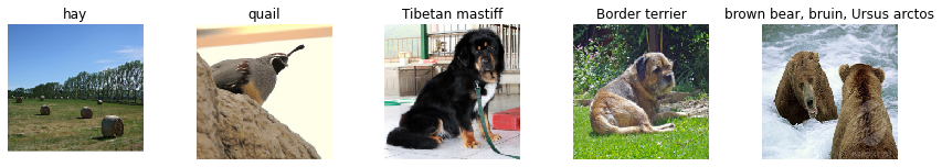
cs231n提供了一些ImageNet ILSVRC 2012里的验证集图片（把目录换到cs231n/datasets/然后运行get_imagenet_val.sh就可以下载这些图片了），由于图片来自于验证集，所以预训练模型并没有见过这些图片，可视化一些图片和它们的真实标签。

from cs231n.data_utils import load_imagenet_val
X, y, class_names = load_imagenet_val(num=5)
plt.figure(figsize=(12, 6))
for i in range(5):
    plt.subplot(1, 5, i + 1)
    plt.imshow(X[i])
    plt.title(class_names[y[i]])
    plt.axis('off')
plt.gcf().tight_layout()

在这里插入图片描述

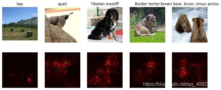
显著图

计算正确类得分关于每个像素的梯度，这个梯度告诉我们，如果某个像素稍微改变了，得分会改变多少。

为了计算显著图[2]，先对梯度取绝对值，然后取3通道中的最大值。所以最后的显著图的大小为(H, W)，并且每个元素都是非负的。
[2] Karen Simonyan, Andrea Vedaldi, and Andrew Zisserman. “Deep Inside Convolutional Networks: Visualising Image Classification Models and Saliency Maps”, ICLR Workshop 2014

提示：PyTorch的gather()方法
回顾Assignment1，有一个从矩阵里选择元素的方法：假设s的大小为(N, C) ，y的大小为(N,) ，包含整数0 <= y[i] < C，那么s[np.arange(N), y] 的大小为(N,)。
在PyTorch中可以使用s.gather(1, y.view(-1, 1)).squeeze()达到同样的效果。关于gather()和squeeze()可以查看文档

# 在PyTorch中使用gather()的例子
def gather_example():
    N, C = 4, 5
    s = torch.randn(N, C)
    y = torch.LongTensor([1, 2, 1, 3])
    print(s)
    print(y)
    print(s.gather(1, y.view(-1, 1)).squeeze())
gather_example()
"""
tensor([[-2.0104, -0.8677, -0.2408, -0.6157,  0.1737],
        [ 0.2832, -0.6364,  0.1452,  1.3739, -0.4388],
        [ 0.6664, -0.1384, -2.7893, -0.5060,  0.1026],
        [-0.7202,  0.5449, -0.2451, -0.9769, -0.3501]])
tensor([1, 2, 1, 3])
tensor([-0.8677,  0.1452, -0.1384, -0.9769])
"""

计算显著图

def compute_saliency_maps(X, y, model):
    """
    Input:
    - X: 输入图像，(N, 3, H, W)
    - y: X的标签，(N,)
    - model: 一个预训练好的CNN模型
    Returns:
    - saliency: 输入X的显著图，(N, H, W)
    """
    # 确保模型在"test"状态
    model.eval()    
    # 需要求输入X的梯度
    X.requires_grad_()
    saliency = None
    
    # 前向传播，取出正确类的得分
    scores = model(X)
    scores = scores.gather(1, y.view(-1, 1)).squeeze()
    # 计算梯度，由于损失要是标量，所以求和
    scores.sum().backward()
    gradient = X.grad
    # 计算显著图
    grads = gradient.abs()
    # 在第1维上比较，也就是红禄蓝三通道上比较
    mx, _ = torch.max(grads, 1)
    saliency = mx.data
    
    return saliency

可视化一些图片的显著图

def show_saliency_maps(X, y):
    # 把X，y转换为Torch张量
    X_tensor = torch.cat([preprocess(Image.fromarray(x)) for x in X], dim=0)
    y_tensor = torch.LongTensor(y)
    # 计算X的显著图
    saliency = compute_saliency_maps(X_tensor, y_tensor, model)
    # 把显著图从Torch张量转化为numpy数组
    saliency = saliency.numpy()
    # 展示原始图片和显著图
    N = X.shape[0]
    for i in range(N):
        plt.subplot(2, N, i + 1)
        plt.imshow(X[i])
        plt.axis('off')
        plt.title(class_names[y[i]])
        plt.subplot(2, N, N + i + 1)
        plt.imshow(saliency[i], cmap=plt.cm.hot)
        plt.axis('off')
        plt.gcf().set_size_inches(12, 5)
    plt.show()
show_saliency_maps(X, y)

可以看到，红色区域的地方大致覆盖了物体，表明模型能够认出物体的大致位置。
在这里插入图片描述

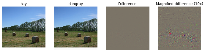
fooling images

可以根据[3]生成"fooling images"：给定一张图片和一个目标类，对图像进行梯度上升，使目标类的得分增大，当网络把图片误分为目标类时停止。
[3] Szegedy et al, “Intriguing properties of neural networks”, ICLR 2014

def make_fooling_image(X, target_y, model):
    """
    生成一张类似于X的图片，但模型会把它认为是target_y
    输入:
    - X: 输入图片，(1, 3, 224, 224)
    - target_y: 一个整数，范围为[0, 1000)
    - model: 一个预训练的CNN模型
    输出:
    - X_fooling: fooling image
    """
    # 初始化图片
    X_fooling = X.clone()
    X_fooling = X_fooling.requires_grad_()    
    learning_rate = 1
    
    # 提示：对于大多数的图像来说，生成一张fooling image需要的迭代次数远远小于100次
    for i in range(100):
        scores = model(X_fooling)
        _,predict = torch.max(scores,1)
        # 如果达到目的，输出迭代次数，跳出循环
        if predict==target_y:
            print("end in %d iterations"%(i))
            break
        
        target_scores = scores[0,target_y]
        target_scores.backward()
        g = X_fooling.grad
        # 在更新梯度之前，先除以梯度的2范数，防止对图像扰动过大
        X_fooling.data += learning_rate*g/g.norm()
        # 由于pytorch的梯度并会叠加，所以需要手动对梯度清零
        X_fooling.grad.data.zero_()
    
    return X_fooling

调用函数生成fooling image

idx = 0
target_y = 6
X_tensor = torch.cat([preprocess(Image.fromarray(x)) for x in X], dim=0)
X_fooling = make_fooling_image(X_tensor[idx:idx+1], target_y, model)
scores = model(X_fooling)
assert target_y == scores.data.max(1)[1][0].item(), 'The model is not fooled!'
# end in 9 iterations

展示原始图片，fooling image还有它们的差异。

X_fooling_np = deprocess(X_fooling.clone())
X_fooling_np = np.asarray(X_fooling_np).astype(np.uint8)
# 原始图像
plt.subplot(1, 4, 1)
plt.imshow(X[idx])
plt.title(class_names[y[idx]])
plt.axis('off')
# fooling image
plt.subplot(1, 4, 2)
plt.imshow(X_fooling_np)
plt.title(class_names[target_y])
plt.axis('off')
# 两者的差异
plt.subplot(1, 4, 3)
X_pre = preprocess(Image.fromarray(X[idx]))
diff = np.asarray(deprocess(X_fooling - X_pre, should_rescale=False))
plt.imshow(diff)
plt.title('Difference')
plt.axis('off')
# 两者的差异乘以10倍
plt.subplot(1, 4, 4)
diff = np.asarray(deprocess(10 * (X_fooling - X_pre), should_rescale=False))
plt.imshow(diff)
plt.title('Magnified difference (10x)')
plt.axis('off')
plt.gcf().set_size_inches(12, 5)
plt.show()

把干草认成了一种鱼，10倍差异图里，相差较大的地方正是干草存在的地方。
在这里插入图片描述

可视化类

从一张随机噪声的图片开始，对目标类执行梯度上升，生成一张能被分为目标类的图片。这个想法是[2]首先提出了的，[4]提供了一些正则化方法来改善生成图像的质量。

𝐼是一张图像，𝑦是目标类，𝑠_𝑦(𝐼)是图像𝐼关于𝑦类的得分。希望生成一张图片 𝐼^∗，使𝑠_𝑦(𝐼^∗)有一个很高的得分，与此同时图像不要变化太大：
在这里插入图片描述
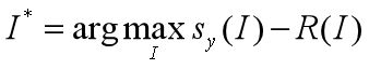
其中，

这个任务中会有两个正则化策略：显示的R(I)正则化和隐式的周期性模糊[4]。
[2] Karen Simonyan, Andrea Vedaldi, and Andrew Zisserman. “Deep Inside Convolutional Networks: Visualising Image Classification Models and Saliency Maps”, ICLR Workshop 2014
[4] Yosinski et al, “Understanding Neural Networks Through Deep Visualization”, ICML 2015 Deep Learning Workshop

def jitter(X, ox, oy):
    """
    对图像进行随机抖动   
    输入：
    - X: 图像，PyTorch张量，(N, C, H, W)
    - ox, oy: 整数，沿w轴和h轴抖动的像素位置
    返回: 一个新的PyTorch张量，(N, C, H, W)
    """
    # 左右互换
    if ox != 0:
        left = X[:, :, :, :-ox]
        right = X[:, :, :, -ox:]
        X = torch.cat([right, left], dim=3)
    # 上下互换
    if oy != 0:
        top = X[:, :, :-oy]
        bottom = X[:, :, -oy:]
        X = torch.cat([bottom, top], dim=2)
    return X

可视化类函数

import math
def create_class_visualization(target_y, model, dtype, **kwargs):
    """
    生成一张图片，最大化它在预训练模型上的得分
    输入:
    - target_y: 目标类，整数，范围为[0, 1000)
    - model:预训练好的CNN模型
    - dtype: Torch数据类型
    Keyword arguments:
    - l2_reg: L2正则化参数
    - learning_rate: 学习率
    - num_iterations: 总共迭代多少次
    - blur_every: 迭代多少次进行一次平滑（作为隐式正则化）
    - max_jitter: 抖动（隐式正则化）多少次
    - show_every: 多少次迭代后展示中间结果
    """
    model.type(dtype)
    l2_reg = kwargs.pop('l2_reg', 1e-3)
    learning_rate = kwargs.pop('learning_rate', 25)
    num_iterations = kwargs.pop('num_iterations', 100)
    blur_every = kwargs.pop('blur_every', 10)
    max_jitter = kwargs.pop('max_jitter', 16)
    show_every = kwargs.pop('show_every', 25)
    
    # 随机初始化PyTorch张量作为输入
    img = torch.randn(1, 3, 224, 224).mul_(1.0).type(dtype).requires_grad_()
    # 画图布局所需数据
    img_num = 0
    # 画图总共有几行
    rows = math.ceil(num_iterations/show_every/3)
    
    for t in range(num_iterations):
        # 随机抖动会得更好的结果
        ox, oy = random.randint(0, max_jitter), random.randint(0, max_jitter)
        img.data.copy_(jitter(img.data, ox, oy))
        
        # 计算得分和损失
        score = model(img)[0,target_y]
        loss = score + learning_rate*img.norm()**2
        score.backward()
        # 梯度上升
        img.data += img.grad
        img.grad.zero_()
        
        # 反随机抖动
        img.data.copy_(jitter(img.data, -ox, -oy))
        # 生成图像像素的上限为hi，下限为lo，区间大约是[-2,3]
        for c in range(3):
            lo = float(-SQUEEZENET_MEAN[c] / SQUEEZENET_STD[c])
            hi = float((1.0 - SQUEEZENET_MEAN[c]) / SQUEEZENET_STD[c])
            img.data[:, c].clamp_(min=lo, max=hi)
        # 周期性模糊图像
        if t % blur_every == 0:
            blur_image(img.data, sigma=0.5)        
        
        # 周期性地展示图片
        if t == 0 or (t + 1) % show_every == 0 or t == num_iterations - 1:
            # 计算图片位置
            img_num += 1
            plt.subplot(rows,3,img_num)
            # 展示图片
            plt.imshow(deprocess(img.clone().cpu()))
            class_name = class_names[target_y]
            plt.title('%s\nIteration %d / %d' % (class_name, t + 1, num_iterations))
            plt.gcf().set_size_inches(14, 10)
            plt.axis('off')
    plt.show()
    return deprocess(img.cpu())

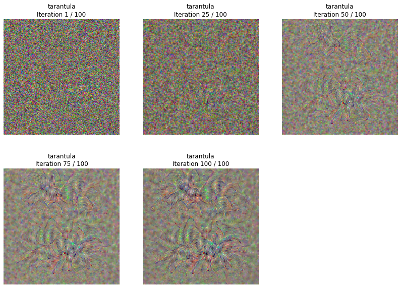
生成一张狼蛛图片:

# dtype = torch.FloatTensor
dtype = torch.cuda.FloatTensor
model.type(dtype)
target_y = 76 # Tarantula狼蛛
out = create_class_visualization(target_y, model, dtype)

在这里插入图片描述
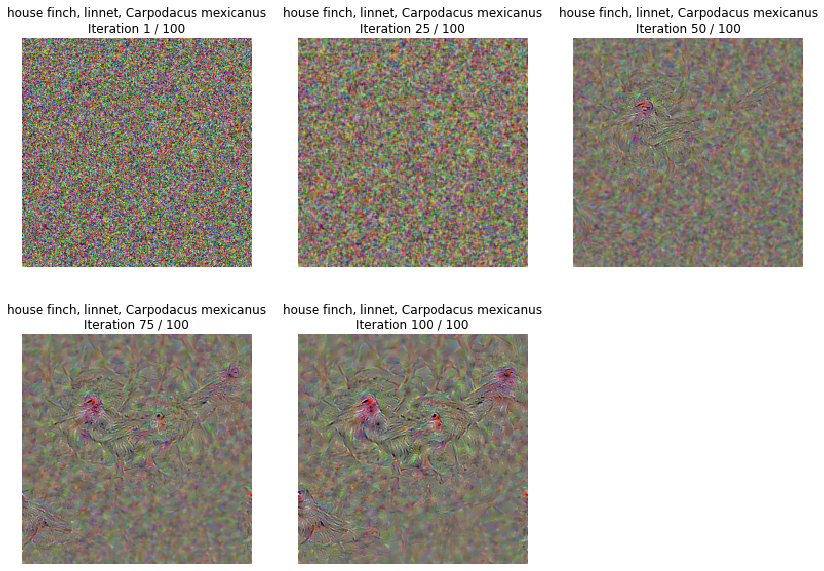
尝试对其他类进行类可视化，能看到一点鸟的样子

target_y = 12 # linnet红雀
print(class_names[target_y])
X = create_class_visualization(target_y, model, dtype)

在这里插入图片描述