


4.5线性回归
线性回归是解决回归问题的常用模型。
实例:简单线性回归
def skLearn13():

    '''

    线性回归

    :return:

    '''

    #简单的一元一次方程

    #斜率为a,截距为b

    #y=ax+b

    #创建线性数据

    rng = np.random.RandomState(0)

    x = 10 * rng.rand(50)

    y = 2*x - 5 + rng.randn(50)

    #绘制数据集

    plt.scatter(x,y)


    #使用线性回归模型

    from sklearn.linear_model import LinearRegression

    model = LinearRegression(fit_intercept=True)

    #拟合数据

    model.fit(x[:,np.newaxis],y)

    #获取训练的斜率和截距

    print(model.coef_)

    print(model.intercept_)

    #构建测试数据

    xtest = np.linspace(0,10,1000)

    ymodel = model.predict(xtest[:,np.newaxis])

    #绘制预测线

    plt.plot(xtest,ymodel)

    #显示图片

    plt.show()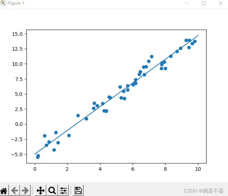
实例2:多项式基函数
将线性回归模型转换为非线性回归模型。
y=a0+a1x1+a2x2+a3x3………
将一个变量x,转换为多维的x1,x2,x3等;
def skLearn14():

    '''

    多项式基函数

    :return:

    '''

    from sklearn.preprocessing import  PolynomialFeatures

    x = np.array([2,3,4])

    print(x)

    poly = PolynomialFeatures(3,include_bias=False)

    #转换为多维数据

    #获取1,2,3次方数据矩阵

    x_trans = poly.fit_transform(x[:,np.newaxis])

    print(x_trans)


    #使用管道,组合多个操作

    from sklearn.pipeline import make_pipeline

    from sklearn.linear_model import  LinearRegression

    #使用5次方多项式

    model = make_pipeline(PolynomialFeatures(5),LinearRegression())


    #构建数据

    rng = np.random.RandomState(1)

    x_data = rng.rand(50) * 10

    y_data = np.sin(x_data) + 0.2 * rng.randn(50)

    #拟合数据

    model.fit(x_data[:,np.newaxis],y_data)

    #预测数据

    x_test = np.linspace(0,10,1000)

    y_model = model.predict(x_test[:,np.newaxis])


    #绘制数据图及预测图

    plt.scatter(x_data,y_data)

    plt.plot(x_test,y_model)

    #显示图片

    plt.show()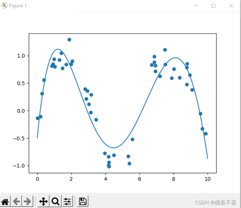
实例3:正则化
当基函数过于灵活,相邻基函数相互影响会导致模型过拟合。为了抑制模型波动,引入正则化机制。常用的正则化:岭回归;Lasso正则化
注意:Lasso倾向于构建稀疏矩阵,将模型系数置为0,所以效果差异大。
def skLearn15():

    '''

    正则化,避免多项式次数过多导致过拟合

    :return:

    '''

    #使用管道,组合多个操作

    from sklearn.pipeline import make_pipeline

    from sklearn.preprocessing import PolynomialFeatures

    from sklearn.linear_model import  LinearRegression

    #使用5次方多项式

    model = make_pipeline(PolynomialFeatures(10),LinearRegression())

    #构建数据

    rng = np.random.RandomState(1)

    x_data = rng.rand(50) * 30

    y_data = np.sin(x_data) + 0.2 * rng.randn(50)

    #拟合数据

    model.fit(x_data[:,np.newaxis],y_data)

    #预测数据

    x_test = np.linspace(0,30,1000)

    y_model = model.predict(x_test[:,np.newaxis])


    #使用岭回归

    from sklearn.linear_model import  Ridge

    model_rid = make_pipeline(PolynomialFeatures(10),Ridge(alpha=0.1))

    #拟合数据

    model_rid.fit(x_data[:,np.newaxis],y_data)

    #测试数据

    y_model_rid = model_rid.predict(x_test[:,np.newaxis])


    #使用Lasso正则化

    from sklearn.linear_model import  Lasso

    model_lasso = make_pipeline(PolynomialFeatures(10),Lasso(alpha=0.001))

    #拟合数据

    model_lasso.fit(x_data[:,np.newaxis],y_data)

    #测试数据

    y_model_lasso = model_lasso.predict(x_test[:,np.newaxis])


    #绘制数据图及预测图

    plt.scatter(x_data,y_data)

    plt.plot(x_test,y_model,label='base line',color='k')

    plt.plot(x_test,y_model_rid,label='rid line',color='g')

    plt.plot(x_test,y_model_lasso,label='lasso line',color='r')

    plt.legend()

    #显示图片

    plt.show()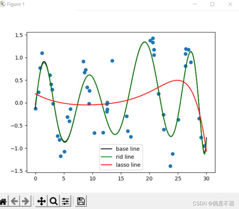


 被折叠的 条评论
为什么被折叠?
被折叠的 条评论
为什么被折叠?
 到【灌水乐园】发言


