机器学习-sklearn练习-1

K近邻算法（knn）

API：sklearn.neighbors.KNeighborsClassifier

KNeighborsClassifier(
n_neighbors=5,
weights='uniform', #uniform neighbors权重相同
algorithm='auto',
leaf_size=30,
p=2, 
metric='minkowski', 
metric_params=None, 
n_jobs=None, 
**kwargs)

n_neighbors：寻找的邻居数，默认是5。也就是K值。一般小于二次根号下（样本数量）

weights：预测中使用的权重函数。可能的取值：‘uniform’：统一权重，即每个邻域中的所有点均被加权。‘distance’：权重点与其距离的倒数，在这种情况下，查询点的近邻比远处的近邻具有更大的影响力。[callable]：用户定义的函数，该函数接受距离数组，并返回包含权重的相同形状的数组。

algorithm：用于计算最近邻居的算法：“ ball_tree”将使用BallTree,“ kd_tree”将使用KDTree,“brute”将使用暴力搜索。“auto”将尝试根据传递给fit方法的值来决定最合适的算法。注意：在稀疏输入上进行拟合将使用蛮力覆盖此参数的设置。

leaf_size:叶大小传递给BallTree或KDTree。这会影响构造和查询的速度，以及存储树所需的内存。最佳值取决于问题的性质。默认30。

p:闵可夫斯基距离的指标的功率参数。当p = 1时，等效于使用曼哈顿距离和p=2时使用欧氏距离。默认是2。

metric：树使用的距离度量。默认度量标准为minkowski，p = 2等于标准欧几里德度量标准。

metric_params：度量函数的其他关键字参数。

n_jobs：并行计算数

练习

1. 电影类别预测
   训练数据集
   

from sklearn.neighbors import KNeighborsClassifier
import pandas as pd

movies = pd.read_excel("data/movies.xlsx")
# 获取数据所有行和2 3 列
data = movies.iloc[:, 1:3]
target = movies['分类情况']
print(data)
print()
print(target)
knn = KNeighborsClassifier(n_neighbors=5)

# 训练
knn.fit(data,target)
# 预测
x_test = pd.DataFrame({'武打镜头': [100, 42, 75], '接吻镜头': [1, 99, 24]})
print()
print(knn.predict(x_test))

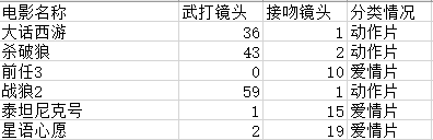
输出结果：
   武打镜头  接吻镜头
0    36     1
1    43     2
2     0    10
3    59     1
4     1    15
5     2    19

0    动作片
1    动作片
2    爱情片
3    动作片
4    爱情片
5    爱情片
Name: 分类情况, dtype: object
['动作片' '爱情片' '动作片']

2. 鸢尾花类别预测

import numpy as np
from sklearn.neighbors import KNeighborsClassifier
from sklearn.datasets import load_iris
from sklearn.preprocessing import StandardScaler

iris = load_iris()
# 输出目标值喝特征值
x = iris['data']
y = iris['target']
# (150,4) 150行数据 4种特征值
print(x.shape)
# 将数据顺序打乱,划分训练集和测试集
index = np.arange(150)
np.random.shuffle(index)
x_train, x_test = x[index[:100]], x[index[100:]]
y_train, y_test = y[index[:100]], y[index[100:]]
# 标准化特征值
std = StandardScaler()
x_train = std.fit_transform(x_train)
x_test = std.transform(x_test)

# 进行训练
knn = KNeighborsClassifier(n_neighbors=5)
knn.fit(x_train, y_train)
# 预测
y_predict = knn.predict(x_test)
print("预测标签为:",y_predict)
print("实际标签为:",y_test)
print("准确率:", knn.score(x_test, y_test))
print("每个样本属于三种类别的可能性", knn.predict_proba(x_test))

输出结果为：
(150, 4)
预测标签为: [2 0 2 2 1 1 2 0 2 0 1 2 1 1 0 2 0 1 0 0 2 2 2 2 0 1 0 2 1 2 0 1 2 0 1 2 1
 1 2 0 0 1 2 0 1 1 2 1 2 1]
实际标签为: [2 0 2 1 1 1 2 0 1 0 1 2 1 1 0 2 0 1 0 0 2 2 2 2 0 1 0 2 1 2 0 1 2 0 1 2 1
 1 2 0 0 1 2 0 1 1 2 1 2 1]
准确率: 0.96
三种类别的可能性 [[0.  0.  1. ]
 [1.  0.  0. ]
 [0.  0.  1. ]
 [0.  0.4 0.6]
 ....

3.手写数字识别
mnist手写集数据
链接：https://pan.baidu.com/s/1_-tkSFZJyy_ReDgbLBrOwA
提取码：1234

import numpy as np
import cv2
from  sklearn.neighbors import KNeighborsClassifier
from sklearn.model_selection import train_test_split
from sklearn.preprocessing import StandardScaler

# 列表
X = []
# 读取10类各500张图片
for i in range(10):
    for j in range(1, 501):
        digit = cv2.imread(r'C:\Users\cpx\Desktop\digit\mnist_train\%d\mnist_train_%d (%d).png' % (i, i, j))
        # 将图片转换成单通道
        digit = cv2.cvtColor(digit, cv2.COLOR_BGR2GRAY)
        X.append(digit)

# 转换为numpy数组 X.shape（5000,28,28）
X = np.asarray(X)
y = np.asarray([i for i in range(10)]*500)
# 排序目标值
y.sort()
# -1代表自动调整 reshape只能有一个-1
X = X.reshape(5000, -1)

std = StandardScaler()
std.fit_transform(X)
# train_test_split会自动打乱数据
# 为了方便此处不再从测试文件夹取测试数据 直接从X 中拿出部分做测试集
x_train, x_test, y_train, y_test = train_test_split(X, y, test_size=0.25)

# 训练
knn = KNeighborsClassifier()
knn.fit(x_train, y_train)
y_predict = knn.predict(x_test)
score = knn.score(x_test, y_test)
print("准确率为", score)

输出结果：
准确率为 0.9416

交叉验证API

sklearn.model_selection.cross_val_score(estimator, X, y=None, groups=None, scoring=None, cv=’warn’, n_jobs=None, verbose=0, fit_params=None, pre_dispatch=‘2*n_jobs’, error_score=’raise-deprecating’)
参数：
estimator： 需要使用交叉验证的算法
X： 输入样本数据
y： 样本标签
scoring： 交叉验证最重要的就是他的验证方式，选择不同的评价方法，会产生不同的评价结果。
具体可用哪些评价指标，官方已给出详细解释，链接：
https://scikitlearn.org/stable/modules/model_evaluation.html#scoring-parameter
cv:交叉验证折数 

在鸢尾花中应用筛选最适合参数

import numpy as np
from sklearn.neighbors import KNeighborsClassifier
from sklearn.datasets import load_iris
from sklearn.preprocessing import StandardScaler
from sklearn.model_selection import cross_val_score
import matplotlib.pyplot as plt


iris = load_iris()
# 输出目标值喝特征值
x = iris['data']
y = iris['target']
# (150,4) 150行数据 4种特征值
print(x.shape)
# 将数据顺序打乱,划分训练集和测试集
index = np.arange(150)
np.random.shuffle(index)
x_train, x_test = x[index[:100]], x[index[100:]]
y_train, y_test = y[index[:100]], y[index[100:]]
# 标准化特征值
std = StandardScaler()
x_train = std.fit_transform(x_train)
x_test = std.transform(x_test)

# 进行训练
weight = ['distance', 'uniform']
errord = []
erroru = []
for k in range(1, 14):
    for w in weight:
        # 选k在1到14 根号下150≈13
        knn = KNeighborsClassifier(n_neighbors=k, weights=w)
        score = cross_val_score(knn, x, y, scoring='accuracy', cv=6).mean()
        if w == 'uniform':
            erroru.append(1 - score)
        else:
            errord.append(1-score)

plt.plot(np.arange(1, 14), errord, c='red', label='distance')
plt.plot(np.arange(1, 14), erroru, c='blue', label='uniform')
plt.legend()
plt.show()

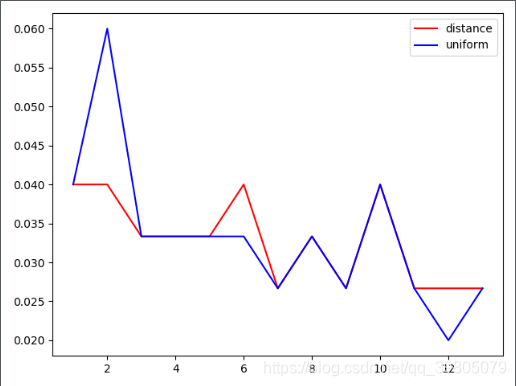
由图像知：当k=12的时候，选uniform可以达到最佳效果

癌症预测
网格搜索 统计等

数据 链接：https://pan.baidu.com/s/1divsvU63ZfOpSK2znO_e7Q 提取码：1234

列：
ID Diagnosis radius_mean texture_mean perimeter_mean area_mean smoothness_mean compactness_mean concavity_mean concave_mean symmetry_mean fractal_mean radius_sd texture_sd perimeter_sd area_sd smoothness_sd compactness_sd concavity_sd concave_sd symmetry_sd fractal_sd radius_max texture_max perimeter_max area_max smoothness_max compactness_max concavity_max concave_max symmetry_max fractal_max

import numpy as np
import pandas as pd
from sklearn.neighbors import KNeighborsClassifier
from sklearn.model_selection import train_test_split
from sklearn.preprocessing import StandardScaler
from sklearn.model_selection import GridSearchCV
from sklearn.metrics import accuracy_score
from sklearn.metrics import classification_report
# 加载数据和提取数据和目标值
cancer = pd.read_csv('./cancer.csv',sep = '\t')
cancer.drop('ID', axis=1, inplace=True)
X = cancer.iloc[:, 1:]
std = StandardScaler()
# 标准化
X = std.fit_transform(X)
y = cancer['Diagnosis']
X_train, X_test, y_train, y_test = train_test_split(X, y, test_size=0.2)
# 网格搜索GridSearchCV进行最佳参数的查找
knn = KNeighborsClassifier()
params = {'n_neighbors': [i for i in range(1, 30)],
          'weights': ['distance', 'uniform'],
          'p': [1, 2]}
# cross_val_score类似
gcv = GridSearchCV(knn, params, scoring='accuracy', cv=6)
gcv.fit(X_train, y_train)
# 查看了GridSearchCV最佳的参数组合
print("best_params：", gcv.best_params_)
print("best_estimator：", gcv.best_estimator_)
print("best_score：", gcv.best_score_)
# 使用GridSearchCV进行预测，计算准确率
y_predict = gcv.predict(X_test)
print("预测值为：", y_predict)
# 精确率两种方式相同
print("准确率为", gcv.score(X_test, y_test))
print("准确率为", accuracy_score(y_test,y_predict))
print()
# 以下统计作用相似
# 交叉表 margins显示行、列和
print(pd.crosstab(index=y_test, columns=y_predict, rownames=['Fact'], colnames=['Predict'],margins=True))
print()
# 分类报告
print(classification_report(y_test, y_predict, target_names=['B', 'M'], labels=['B', 'M']))

输出结果：
best_params： {'n_neighbors': 9, 'p': 2, 'weights': 'distance'}
best_estimator： KNeighborsClassifier(algorithm='auto', leaf_size=30, metric='minkowski',
                     metric_params=None, n_jobs=None, n_neighbors=9, p=2,
                     weights='distance')
best_score： 0.9692397660818713
预测值为： ['M' 'B' 'B' 'M' 'B' 'B' 'B' 'B' 'B' 'B' 'B' 'M' 'B' 'M' 'B' 'M' 'M' 'B'
 'M' 'M' 'M' 'B' 'B' 'B' 'B' 'B' 'B' 'B' 'B' 'M' 'B' 'B' 'B' 'B' 'M' 'M'
 'B' 'B' 'B' 'M' 'B' 'B' 'M' 'B' 'B' 'B' 'B' 'B' 'M' 'B' 'B' 'B' 'M' 'B'
 'M' 'B' 'B' 'M' 'B' 'B' 'B' 'M' 'B' 'M' 'M' 'M' 'B' 'B' 'M' 'M' 'M' 'B'
 'B' 'M' 'M' 'B' 'B' 'M' 'B' 'B' 'B' 'M' 'B' 'B' 'B' 'B' 'M' 'M' 'M' 'B'
 'B' 'B' 'M' 'B' 'M' 'M' 'B' 'M' 'B' 'B' 'M' 'B' 'B' 'B' 'M' 'M' 'M' 'B'
 'B' 'B' 'M' 'M' 'M' 'B']
准确率为 0.9912280701754386
准确率为 0.9912280701754386

Predict   B   M  All
Fact                
B        70   0   70
M         1  43   44
All      71  43  114

              precision    recall  f1-score   support

           B       0.99      1.00      0.99        70
           M       1.00      0.98      0.99        44

    accuracy                           0.99       114
   macro avg       0.99      0.99      0.99       114
weighted avg       0.99      0.99      0.99       114

OneHot编码
又称一位有效编码，其方法是使用N位状态寄存器来对N个状态进行编码，每个状态都由他独立的寄存器位，并且在任意时候，其中只有一位有效。对于每一个特征，如果它有m个可能值，那么经过独热编码后，就变成了m个二元特征。并且，这些特征互斥，每次只有一个激活。因此，数据会变成稀疏的。这样做的好处主要有：

1. 解决了分类器不好处理属性数据的问题
2. 在一定程度上也起到了扩充特征的作用

str类型数据转换和预测
对于字符串类型的特征值可以使用预处理中的API转换成数字编码

preprocessing.OrdinalEncoder（）：能够将字符串转换为数值
preprocessing.LabelEncoder（）：与上相似，但是数据得一列一列传入
preprocessing.OneHotEncoder（）：无法直接对字符串型的类别变量编码，可以将数字转换成01编码
（参数均为二维数组，可以将series加中括号就会变成二维dataframe）
例：

data = salary['education']#series
data = [data]

薪水转换示例
数据示例：

import numpy as np
import pandas as pd
from sklearn.preprocessing import OrdinalEncoder,OneHotEncoder,LabelEncoder
from sklearn.neighbors import KNeighborsClassifier

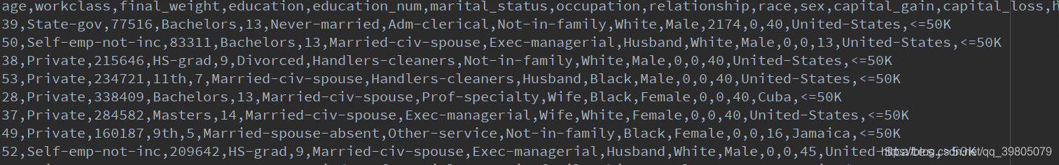
salary = pd.read_csv(r"./salary.txt")
salary.drop(labels=['final_weight', 'education_num', 'capital_gain', 'capital_loss'], axis=1, inplace=True)
X = salary.iloc[:, 0:-1]
y = salary['salary']
ord = OrdinalEncoder()
data = ord.fit_transform(salary)
print(data)
salary_ordinal = pd.DataFrame(data, columns=salary.columns)
print(salary_ordinal)

输出结果：
[[22.  7.  9. ... 39. 39.  0.]
 [33.  6.  9. ... 12. 39.  0.]
 [21.  4. 11. ... 39. 39.  0.]
 ...
 [41.  4. 11. ... 39. 39.  0.]
 [ 5.  4. 11. ... 19. 39.  0.]
 [35.  5. 11. ... 39. 39.  1.]]
        age  workclass  education  ...  hours_per_week  native_country  salary
0      22.0        7.0        9.0  ...            39.0            39.0     0.0
1      33.0        6.0        9.0  ...            12.0            39.0     0.0
2      21.0        4.0       11.0  ...            39.0            39.0     0.0
3      36.0        4.0        1.0  ...            39.0            39.0     0.0
4      11.0        4.0        9.0  ...            39.0             5.0     0.0
...     ...        ...        ...  ...             ...             ...     ...
32556  10.0        4.0        7.0  ...            37.0            39.0     0.0
32557  23.0        4.0       11.0  ...            39.0            39.0     1.0
32558  41.0        4.0       11.0  ...            39.0            39.0     0.0
32559   5.0        4.0       11.0  ...            19.0            39.0     0.0
32560  35.0        5.0       11.0  ...            39.0            39.0     1.0

[32561 rows x 11 columns]