一元多项式回归

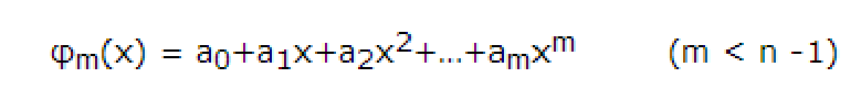
设拟合多项式为φm(x)

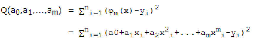
残差平方和

用最小二乘来确定系数a0，a1，…，am，设残差平方和

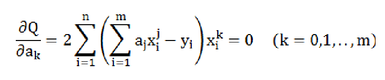
Q对ak求偏导数，并令其等于零，有

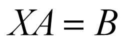
写成矩阵形式为：


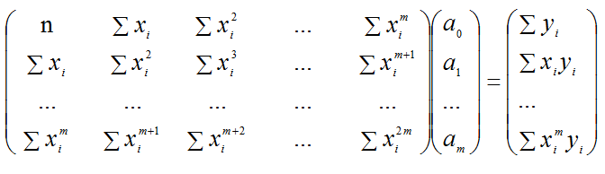
（上面的方程是解别人的图，原址奉上：https://www.cnblogs.com/144823836yj/p/5524610.html ）
接下来就是解线性方程组

增广矩阵法

由于需要构造系数为1，将进行大量浮点运算，况且矩阵的元素肯能很大，会出现大吃小的可能，会引入大量误差

在数据量少，阶数较小时适用
列
x=c(1,2,3,4,5)
y = c(1,1.5,3,4.5,5)
二次多项式拟合增广矩阵

5.0 15.0 55.0 | 15
15.0 55.0 225.0 | 56
55.0 225.0 979.0 | 231
解为 -0.3 ，1.1 ，0.0
x矩阵为非正定矩阵，秩为2，拟合为一次项

逆矩阵法

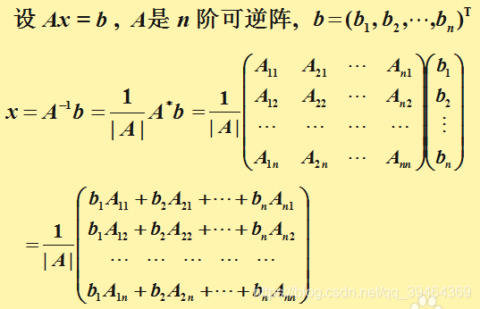
依旧计算量相当大，浮点运算误差影响更大

R代码

三次多项式拟合

x=matrix(c(5.0,	15.0,	55.0,	225.0	,
           15.0,	55.0,	225.0,	979.0	,
           55.0,	225.0,	979.0,	4425.0,	
           225.0,	979.0,	4425.0,	20515.0	),
         nr=4,nc=4)
b=matrix(c(15.0,	56.0,	231.0	,1007.0	),nr=4,nc=1)
c=solve(x)%*%b
a=matrix(c(1.5,-1,0.5),nr=3,nc=1)

> c
           [,1]
[1,]  2.5000000
[2,] -2.8333333
[3,]  1.5000000
[4,] -0.1666667

solve(x)为求x的逆矩阵
solve(x,b)可直接求解xa=b

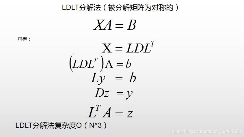
针对对称矩阵有LDLT分解法（LT为L的转置）

java代码

public class CurveFit {
	public static void main(String[] args) {
		double[] x=new double[] {1,2,3,4,5};
		double[] y=new double[] {1,1.5,3,4.5,5};
		
		show(curveFit(x,y,3));
	}
	public static double [] curveFit(double[] x,double[] y,int pow) {
		double[][] matrix=createMatrix(x,y,pow);
		LDLTDCMP(matrix);
		double [] xy=iteration(y,x,pow+1);
		LDLTBKSB(matrix,xy);
		return xy;
	}
	public static double[][] createMatrix(double[] x,double[] y,int pow) {
		double [] xx=iteration(x,x,2*pow);
		double[][] matrix=new double[pow+1][pow+1];
		matrix[0][0]=x.length;
		for(int i=0;i<pow+1;i++) {
			for(int k=0;k<pow+1;k++) {
				if(i+k>0) {
					matrix[i][k]=xx[i+k-1];
				}
			}
		}
	
		return matrix;
		
	}
	public static double[] iteration(double[] start,double [] value,int count) {
		double[] itr = null;
		double[] ret = new double [count];
		for(int i=0;i<count;i++) {
			if(i==0) {
				itr=start.clone();
			}else {
				itr=mul(itr,value);
			}
			ret[i]=sum(itr);
		}
		return ret;
	}
	public static double[] mul(double[] a,double[] b) {
		double[] c=a.clone();
		if(a.length==b.length) {
			for(int i=0;i<a.length;i++) {
				c[i]*=b[i];
			}
		}
		return c;
	}
	public static double sum(double[] a) {
		double ret=0;
		for(int i=0;i<a.length;i++) {
			ret+=a[i];
		}
		return ret;
	}
	
	public static void LDLTDCMP ( double [][]a)
	{
	    int k=0,m=0,i=0,n=a.length;
	    for (k = 0; k < n; k++)
	    {
	        for (m = 0; m < k; m++) {
	        	a[k][k] = a[k][k] - a[m][k] * a[k][m];
	        }  
	        if (a[k][k] == 0)
	        {
	            return;
	        }
	        for (i = k + 1; i < n; i++)
	        {
	            for (m = 0; m < k; m++)
	                a[k][i] = a[k][i] - a[m][i] * a[k][m];
	            a[i][k] = a[k][i] / a[k][k];
	        }
	    }
	}

	public static void LDLTBKSB ( double[][]a, double []b)
	{
	    int i;
	    int k;
	    int n=a.length;
	    for (i = 0; i < n; i++){
	        for (k = 0; k < i; k++)
	            b[i] = b[i] - a[i][k] * b[k];
	    }
	    for (i = n - 1; i >= 0; i--){	       
	        b[i] = b[i] / a[i][i];
	        for (k = i + 1; k < n; k++)
	            b[i] = b[i] - a[k][i] * b[k];
	    }
	}
	
    public static void show(double[][] array) {
    	for(int i=0;i<array.length;i++) {
    		double[] itme=array[i];
    		for(double out:itme) {
    			System.out.print(out+"\t");
    		}
    		System.out.println();
    	}System.out.println();
    };
    public static void show(double[] array) {
    	for(double out:array) {
    		System.out.print(out+"\t");
    	}
    	System.out.println();
    	System.out.println();
    }
}

LDLTDCMP为矩阵分解 ，LDLTBKSB为求解，两个方法是网上看见的，非常精炼，自愧不如，拿来就用
运行结果：

2.500000000000047 -2.833333333333396 1.5000000000000235 -0.1666666666666693

R语言多项式回归

x=c(1,2,3,4,5)
y = c(1,1.5,3,4.5,5)
xy=data.frame(x=x,y=y) 
#model <- lm(xy$y ~ poly(x,3))
model <- lm(xy$y ~  x + I(x^2) + I(x^3))

回归模型

> model

Call:
lm(formula = xy$y ~ x + I(x^2) + I(x^3))

Coefficients:
(Intercept)            x       I(x^2)       I(x^3)  
     2.5000      -2.8333       1.5000      -0.1667   

模型摘要

> summary(model)

Call:
lm(formula = xy$y ~ x + I(x^2) + I(x^3))

Residuals:
         1          2          3          4          5 
 3.052e-16 -1.221e-15  1.831e-15 -1.221e-15  3.052e-16 
Coefficients:
              Estimate Std. Error    t value Pr(>|t|)    
(Intercept)  2.500e+00  1.256e-14  1.990e+14 3.20e-15 ***
x           -2.833e+00  1.642e-14 -1.726e+14 3.69e-15 ***
I(x^2)       1.500e+00  6.094e-15  2.461e+14 2.59e-15 ***
I(x^3)      -1.667e-01  6.729e-16 -2.477e+14 2.57e-15 ***
---
Signif. codes:  0 ‘***’ 0.001 ‘**’ 0.01 ‘*’ 0.05 ‘.’ 0.1 ‘ ’ 1

Residual standard error: 2.554e-15 on 1 degrees of freedom
Multiple R-squared:      1,	Adjusted R-squared:      1 
F-statistic: 6.39e+29 on 3 and 1 DF,  p-value: 9.196e-16

p值9.196e-16接近于0说明完美拟合。

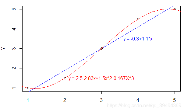
拟合图像

x=c(1,2,3,4,5)
y = c(1,1.5,3,4.5,5)

f1=function(x){
  -0.3+1.1*x
}
f3=function(x){
  2.5-2.83*x+1.5*x^2-0.167*x^3
}
plot(x,y)
curve(f1,from=0,to=6,col="blue",add=T)
curve(f3,from=0,to=6,col="red",add=T)

text(4,3.5, "y = -0.3+1.1*x",col="blue")
text(3,1.5, "y = 2.5-2.83x+1.5x^2-0.167X^3",col="red")

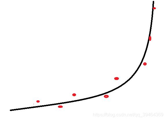
过拟合问题

1.拟合度高并不代表模型最优

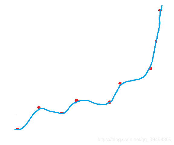
2.拟合度低并不代表模型很差