Cousera-AndrewNg(吴恩达)机器学习笔记--第二周编程作业(线性回归)

Coursera-AndrewNg线性回归编程作业

准备工作

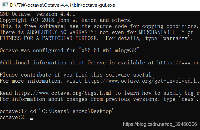
从网站上将编程作业要求下载解压后，在Octave中使用cd命令将搜索目录移动到编程作业所在目录中，博主的所有数据文件都在桌面，路径移动如下图所示：

单变量线性回归

STEP1 PLOTTING THE DATA

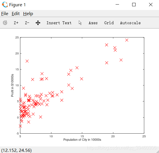
在处理数据之前，可以通过离散的点来描绘它，在一个2D的平面里，把ex1data1中的内容读取到X变量和y变量中，用m表示数据长度。代码如下：

data = load('ex1data1.txt');
X = data(:,1);
y = data(:,2);
m = length(y);

接下来通过图像描绘出来。

plotData(X,y);
ylabel('Profit in $10,000s');
xlabel('Population of City in 10,000s');

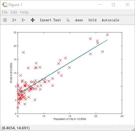
得到的图像如图所示，就是原始的数据的直观表示。

STEP2 GRADIENT DESCENT

然后通过梯度下降对参数θ进行线性回归。
依照课程所得出的步骤方法

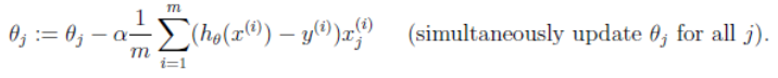
迭代更新
计算θ值函数computeCost.m:

function J = computeCost(X,y,theta)
%COMPUTECOST compute cost for linear regression
%J=COMPUTECOST(X,y,theta)  computes the cost of using theta as the parameter for linear regression to fit the data points in X and y
%Initialize some useful values
m = length(y); %number of training examples

%return the following variables correctly
J=0;

%Compute the cost of a particular choice of theta
%set J to the cost

%===========YOUR CODE HERE============
prediction = X*theta;
sqr=(prediction-y).^2;
J=1/(2*m)*sum(sqr)
%=======================================
end

梯度下降函数gradientDescent.m:

function[theta,J_history]=gradientDescent(X,y,theta,alpha,num_iters)
%GRADIENTDESCENT Performs gradient descent to learn theta
%   theta = GRADIENTDESCENT(X, y, theta, alpha, num_iters) updates theta by 
%   taking num_iters gradient steps with learning rate alpha

% Initialize some useful values
m = length(y); % number of training examples
J_history = zeros(num_iters, 1);

for iter = 1:num_iters
%======================YOU CODE HERE========================
 % Instructions: Perform a single gradient step on the parameter vector theta
 prediction = X * theta;
 error = prediction - y;
 sums = X' * error;
 delta = 1 / m * sums; 
 theta = theta - alpha * delta;
 %============================================================

% Save the cost J in every iteration
J_history(iter) = computeCost(X, y, theta);

end

绘图函数plotData(x,y):

function plotData(x, y)
%PLOTDATA Plots the data points x and y into a new figure
%   PLOTDATA(x,y) plots the data points and gives the figure axes labels of population and profit.

%====================YOU CODE HERE=========================
plot(x,y,'rx','MarkerSize',10);
ylabel('Profit in $10,000s');
xlabel('Population of City in 10,000s');
%============================================================
end

根据以上函数，进行线性回归：

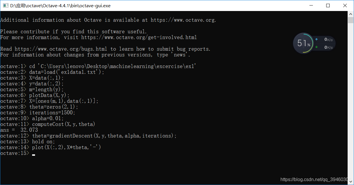
代码文本如下：

octave:1> cd 'C:\Users\lenovo\Desktop\machinelearning\excercise\ex1'
octave:2> data=load('ex1data1.txt');
octave:3> X=data(:,1);
octave:4> y=data(:,2);
octave:5> m=length(y);
octave:6> plotData(X,y);
octave:7> X=[ones(m,1),data(:,1)];
octave:8> theta=zeros(2,1);
octave:9> iterations=1500;
octave:10> alpha=0.01;
octave:11> computeCost(X,y,theta)
ans =  32.073
octave:12> theta=gradientDescent(X,y,theta,alpha,iterations);
octave:13> hold on;
octave:14> plot(X(:,2),X*theta,'-')

结果如如图所示：

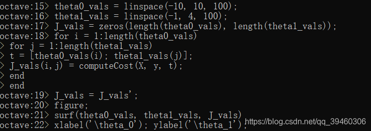
% Grid over which we will calculate J
theta0_vals = linspace(-10, 10, 100);
theta1_vals = linspace(-1, 4, 100);
% initialize J_vals to a matrix of 0's
J_vals = zeros(length(theta0_vals), length(theta1_vals));

% Fill out J_vals
for i = 1:length(theta0_vals)
       for j = 1:length(theta1_vals)
       t = [theta0_vals(i); theta1_vals(j)]; 
       J_vals(i,j) = computeCost(X, y, t);
       end
 end

% Because of the way meshgrids work in the surf command, we need to transpose J_vals before calling surf, or else the axes will be flipped
J_vals = J_vals';
figure;
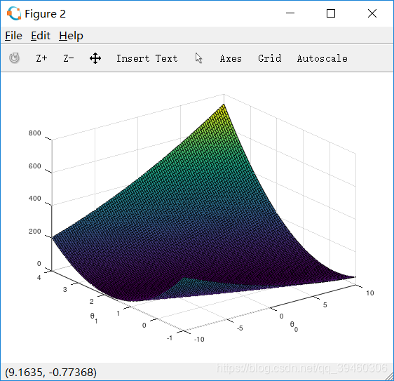
surf(theta0_vals, theta1_vals, J_vals)
xlabel('\theta_0'); ylabel('\theta_1');

结果如图所示：

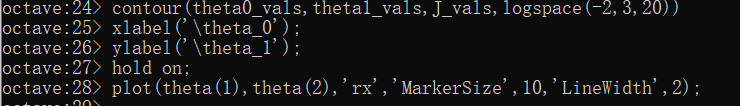
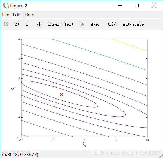
根据数据绘制等高线图：

代码文本如下：

% Contour plot
figure;
% Plot J_vals as 15 contours spaced logarithmically between 0.01 and 100
contour(theta0_vals, theta1_vals, J_vals, logspace(-2, 3, 20))
xlabel('\theta_0'); ylabel('\theta_1');
hold on;
plot(theta(1), theta(2), 'rx', 'MarkerSize', 10, 'LineWidth', 2);

结果图如图所示：