


文章目录
- 4.1 SIAMCAT包的基本用法
- 4.1.1 SIAMCAT basic vignette
- 4.1.2 SIAMCAT confounder example
- 4.1.3 SIAMCAT holdout testing
- 4.1.4 SIAMCAT input
- Introduction
- [Loading your data into R](https://bioconductor.org/packages/release/bioc/vignettes/SIAMCAT/inst/doc/SIAMCAT_read-in.html#loading-your-data-into-r)
- [Creating a siamcat-class object](https://bioconductor.org/packages/release/bioc/vignettes/SIAMCAT/inst/doc/SIAMCAT_read-in.html#creating-a-siamcat-class-object)
- 4.1.5 SIAMCAT meta-analysis
- 4.1.6 SIAMCAT ML pitfalls
论文:Wirbel, J., Zych, K., Essex, M. et al. Microbiome meta-analysis and cross-disease comparison enabled by the SIAMCAT machine learning toolbox. Genome Biol 22, 93 (2021). https://doi.org/10.1186/s13059-021-02306-1
Github代码:https://github.com/zellerlab/siamcat_paper
相关数据:https://doi.org/10.5281/zenodo.4454489
论文要点:
- **导致过拟合的原因:**supervised feature filtering 和naive splitting of dependent samples。
- supervised feature filtering :特征选择过程中考虑了标签信息。
- naive splitting of dependent samples:注意同一个个体不同采样时间点的情况。
-
如何解决spurious association和reproducibility issues的问题?——control augmention.
-
模型自省(model introspection):微生物组变化到底是疾病特异性的,还是具有普遍性的失调?
4.1 SIAMCAT包的基本用法
测试目录:F:\Zhaolab2020\gut-brain-axis\metaAD\2021GB_SIAMCAT\testwork
注意:最好使用R4版本。
4.1.1 SIAMCAT basic vignette
标签设置:
label.crc.zeller <- create.label(meta=meta.crc.zeller,
    label='Group', case='CRC')

##函数
create.label(label, case,
    meta=NULL, control=NULL,
    p.lab = NULL, n.lab = NULL,
    remove.meta.column=FALSE,
    verbose=1)
#label是用于创建标签的命名向量和metadata列的名字。
#verbose:整数,用于控制输出。0表示不输出,1表示只输出进程或者成功相关信息,2表示正常水平的信息,3用于debug information. 默认为1。
将数据导入siamcat:
sc.obj <- siamcat(feat=feat.crc.zeller,
    label=label.crc.zeller,
    meta=meta.crc.zeller)

##SIAMCAT constructor function
siamcat(..., feat=NULL, label=NULL, meta=NULL,
    phyloseq=NULL, validate=TRUE, verbose=3)
特征过滤
sc.obj <- filter.features(sc.obj,
                          filter.method = 'abundance',
                          cutoff = 0.001)
###Perform unsupervised feature filtering.
filter.features(siamcat, filter.method = "abundance",
    cutoff = 0.001, rm.unmapped = TRUE,
    feature.type='original', verbose = 1)
###filter.method包括 c('abundance', 'cum.abundance', 'prevalence', 'variance'),默认是'abundance'。
###cutoff: float, abundace, prevalence, or variance cutoff, defaults to 0.001
###rm.unmapped: 是否去掉unmapped, 默认为去掉。
###feature.type: "original", "filtered", or "normalized"。
特征选择方法:
- ‘abundace’ - remove features whose maximum abundance is never above the threshold value in any of the samples. 去掉再任何样本中最大丰度均不超过阈值的特征。
- ‘cum.abundance’ - remove features with very low abundance in all samples, i.e. those that are never among the most abundant entities that collectively make up (1-cutoff) of the reads in any sample。去掉在所有样本中丰度都很低的特征。
- ‘prevalence’ - remove features with low prevalence across samples, i.e. those that are undetected (relative abundance of 0) in more than 1 - cutoff percent of samples. 流行度。
- ‘variance’ - remove features with low variance across samples, i.e. those that have a variance lower than cutoff。去掉方差很小的特征。
关联检测:
sc.obj <- check.associations(
    sc.obj,
    sort.by = 'fc',
    alpha = 0.05,
    mult.corr = "fdr",
    detect.lim = 10 ^-6,
    plot.type = "quantile.box",
    panels = c("fc", "prevalence", "auroc"))


##Check and visualize associations between features and classes
check.associations(siamcat, fn.plot=NULL, color.scheme = "RdYlBu",
    alpha =0.05, mult.corr = "fdr", sort.by = "fc",
    detect.lim = 1e-06, pr.cutoff = 1e-6, max.show = 50,
    plot.type = "quantile.box",
    panels = c("fc","auroc"), prompt = TRUE,
    feature.type = 'filtered', verbose = 1)
##fn.plot: string, filename for the pdf-plot.
##alpha:float, significance level, defaults to 0.05
##mult.corr: string, multiple hypothesis correction method, see p.adjust, defaults to "fdr"
##sort.by: string, sort features by p-value ("p.val"), by fold change ("fc") or by prevalence shift ("pr.shift")
##detect.lim: 对数变换前的伪计数。
##pr.cutoff: float, cutoff for the prevalence computation(流行度计算), defaults to 1e-06
##max.show:相关特征的数目。
##plot.type:制定丰度的绘图方式。c("bean", "box", "quantile.box", "quantile.rect")
##panels:c("fc", "auroc", "prevalence")
关联检测中值得注意的内容:
-
多重假设检验矫正的原理是什么?Bonferroni(
p*(1/n)) 和 FDR(**Benjaminiand Hochberg: **α*k/m)的区别是什么?https://zhuanlan.zhihu.com/p/51546651 -
c(“bean”, “box”, “quantile.box”, “quantile.rect”)等绘图方式分别是什么含义?参考F:\Zhaolab2020\gut-brain-axis\metaAD\2021GB_SIAMCAT\testwork测试结果。
-
丰度图旁边的panels名字:c(“fc”, “auroc”, “prevalence”)分别是什么意思? 如何绘制的?
- Significance as computed by a Wilcoxon test followed by multiple hypothesis testing correction. 非参数样本检验,基于样本的秩次排列,将两独立样本组的非正态样本值进行比较。【注意:参数检验假定数据服从某分布(一般为正态分布),通过样本参数的估计量(x±s)对总体参数(μ)进行检验,比如t检验、u检验、方差分析。非参数检验不需要假定总体分布形式,直接对数据的分布进行检验,比如,卡方检验和wilcoxon秩和检验。】
- AUROC (Area Under the Receiver Operating Characteristics Curve) as a non-parameteric measure of enrichment (corresponds to the effect size of the Wilcoxon test). 【相关名词: 敏 感 性 s e n s i t i v i t y = T P T P + F N 敏感性sensitivity=\frac{TP}{TP+FN} 敏感性sensitivity=TP+FNTP, 特异性 s p e c i f i c i t y = T N F P + T N specificity=\frac{TN}{FP+TN} specificity=FP+TNTN, Wilcoxon-Mann-Whitney test的U statistic 证明有时间再仔细研究。参考:https://zhuanlan.zhihu.com/p/326327644】
- The generalized Fold Change (gFC) is a pseudo fold change which is calculated as geometric mean of the differences between the quantiles for the different classes found in the label. 【充分利用到Fold change的后验分布的方差的信息,参考https://kevinzjy.github.io/2017/05/20/170520-Paper-GFOLD/】
- The prevalence shift between the two different classes found in the label. 【应该就是本来的意思:流行度。在样本中出现的频率。】
Confounder Testing(混杂因素测试):
sc.obj <- check.confounders(
    sc.obj,
    fn.plot = 'confounder_plots.pdf',
    meta.in = NULL,
    feature.type = 'filtered'
)

##Check for potential confounders in the metadata
check.confounders(siamcat, fn.plot, meta.in = NULL, verbose = 1)
##meta.in: vector, specific metadata variable names to analyze, defaults to NULL (all metadata variables will be analyzed)
##详情:该函数检查分类标签与metadata中潜在的混在因素(例如:age, sex 或者BMI)之间的关联。统计检验包括Fisher's extact text或者Wilcoxon test, 关联使用barplot或者Q-Q plot来可视化, 可视化形式取决于metadata的类型。
##另外,其通过条件熵(conditional entropy and association)来评估metadata variables之间的关联。使用广义线性模型(generalized linear models)来评估标签与metadata variable之间的关联,提供一个关联热图和合适的定量箱线图(boxplots)。
相关问题:
- Fisher’s extact test或者Wilcoxon test的区别是什么? 【Fisher’s extact test(用于离散型变量): 用于分析列联表的统计显著性检验方法。Wilcoxon检验(用于连续型变量):非参数样本检验,基于样本的秩次排序,将两独立样本组的非正态样本值进行比较。】
- Q-Q plot是什么形式的?有什么意义?怎么使用ggplot2绘制?【quantile-quantile (QQ) plot: 比较累计分布函数来判断两组数据是否服从同一分布。】
- 什么是条件熵(conditional entropy)?【**条件熵(Conditional Entropy):**表示两个随机变量X和Y,在已知Y的情况下对随机变量X的不确定性,称之为条件熵H(X|Y)。】
- 什么是广义线性模型(generalized linear models)?如何使用R来实现?【**广义线性模型**就是把自变量的线性预测函数当作因变量的估计值。很多模型都是基于广义线性模型的,例如,传统的线性回归模型,最大熵模型,Logistic回归,softmax回归。】
- 关联热图(heatmaps)和合适的定量箱线图(boxplots)是什么意思?【参考测试目录:F:\Zhaolab2020\gut-brain-axis\metaAD\2021GB_SIAMCAT\testwork】。
- 方差(variance)解释部分是什么意思? 为什么左上角有很多特征的变量可能是标签关联的混杂因素?如何解释呢?
数据归一化(Data Normalization):
sc.obj <- normalize.features(
    sc.obj,
    norm.method = "log.unit",
    norm.param = list(
        log.n0 = 1e-06,
        n.p = 2,
        norm.margin = 1
    )
)

##Perform feature normalization
normalize.features(siamcat,
    norm.method = c("rank.unit", "rank.std",
        "log.std", "log.unit", "log.clr"),
    norm.param = list(log.n0 = 1e-06, sd.min.q = 0.1,
        n.p = 2, norm.margin = 1),
    feature.type='filtered',
    verbose = 1)
##norm.method: c('rank.unit', 'rank.std', 'log.std', 'log.unit', 'log.clr')
##norm.param: 设置不同归一化方法的参数。
##feature.type:"original", "filtered", or "normalized".
说明:
- 5种归一化方法:
rank.unit(将特征转化为秩,然后归一化每一列);rank.std(将特征转化为ranks, 然后进行z-score归一化);log.clr(中心对数比例转化);log.std(对数转化,然后z-score归一化);log.unit(对数变化,然后归一化)。 - 归一化参数:
rank.unit不需要任何其他参数;rank.std(sd.min.q加上的最小方差);log.clr(log.n0是对数变换前的伪计数);log.std(log.n0和sd.min.q);log.unit(参数包括log.n0,np和norm.margin。n.p指定了使用的向量范数,norm.margin指定标准化的边界,其中1表示对特征标准化,2表示对样本,3表示全局最大的标准化。)
准备交叉验证(Prepare Cross-Validation):进行两次重复的5-折交叉验证。
sc.obj <-  create.data.split(
    sc.obj,
    num.folds = 5,
    num.resample = 2
)

##Split a dataset into training and a test sets.
create.data.split(siamcat, num.folds = 2, num.resample = 1,
    stratify = TRUE, inseparable = NULL, verbose = 1)
##inseparable: 不可分割的元数据变量中的名字。
训练模型(Model Training):
sc.obj <- train.model(
    sc.obj,
    method = "lasso"
)

##This function trains the a machine learning model on the training data
train.model(siamcat,
    method = c("lasso", "enet", "ridge", "lasso_ll",
        "ridge_ll", "randomForest"),
    stratify = TRUE, modsel.crit = list("auc"),
    min.nonzero.coeff = 1, param.set = NULL,
    perform.fs = FALSE,
    param.fs = list(thres.fs = 100, method.fs = "AUC", direction='absolute'),
    feature.type='normalized',
    verbose = 1)
##method: 训练模型的方法包括c('lasso', 'enet', 'ridge', 'lasso_ll', 'ridge_ll', 'randomForest')。
##modsel.crit: 模型选择的标准包括c('auc', 'f1', 'acc', 'pr')。
##min.nonzero.coeff:模型(仅对于'lasso', 'ridge', and 'enet')中应该出现的最小非零系数的整数,默认为1。
##param.set:参数设置,可能包括:cost-for lasso_ll and ridge_ll; alpha-for enet; ntree and mtry - for RandomForest)
##perform.fs: 设定是否进行特征选择。
##param.fs: 用于特征选择的参数,必须包括(thres.fs--用于特征选择的阈值;method.fs: 用于特征选择的方法,包括AUC、gFC和Wilcoxon;direction:对于AUC和gFC而言,最关联特征的方向,可能是absolute, positive或者negative。
机器学习模型和参数来自**mlr包。对于需要额外超参数的机器学习方法,最有超参数可以通过mlr**包的tuneParams函数来实现。
- ‘lasso’, ‘enet’, and ‘ridge’ use the ‘classif.cvglmnet’ Learner,
- ‘lasso_ll’ and ‘ridge_ll’ use the ‘classif.LiblineaRL1LogReg’ and the 'classif.LiblineaRL2LogReg’ Learners respectively
- ‘randomForest’ is implemented via the ‘classif.randomForest’ Learner.
用于特征选择的函数:
-
‘AUC’ - computes the Area Under the Receiver Operating Characteristics Curve for each single feature and selects the top param.fs$thres.fs, e.g. 100 features
-
‘gFC’ - computes the generalized Fold Change (see check.associations) for each feature and likewise selects the top param.fs$thres.fs, e.g. 100 features
-
Wilcoxon - computes the p-Value for each single feature with the Wilcoxon test and selects features with a p-value smaller than param.fs$thres.fs
相关问题:
- 模型训练方法c(‘lasso’, ‘enet’, ‘ridge’, ‘lasso_ll’, ‘ridge_ll’, ‘randomForest’)等的原理是什么?如何使用python或者R语言来实现?
- LASSO算法理论介绍:https://blog.youkuaiyun.com/slade_sha/article/details/53164905。 min β 1 2 ∥ y − ∑ i = 1 n x i β i ∥ 2 2 + λ ∥ β ∥ 1 \min _{\beta} \frac{1}{2}\left\|\mathbf{y}-\sum_{i=1}^{n} \mathbf{x}_{i} \beta_{i}\right\|_{2}^{2}+\lambda\|\beta\|_{1} minβ21∥y−∑i=1nxiβi∥22+λ∥β∥1
- 弹性网络(Elastic Net):https://blog.youkuaiyun.com/qq_21904665/article/details/52315642。 m i n w 1 2 n s a m p l e s ∣ ∣ X w − y ∣ ∣ 2 2 + α ρ ∣ ∣ w ∣ ∣ 1 + α ( 1 − ρ ) 2 ∣ ∣ w ∣ ∣ 2 2 \underset{w}{min\,} { \frac{1}{2n_{samples}} ||X w - y||_2 ^ 2 + \alpha \rho ||w||_1 +\frac{\alpha(1-\rho)}{2} ||w||_2 ^ 2} wmin2nsamples1∣∣Xw−y∣∣22+αρ∣∣w∣∣1+2α(1−ρ)∣∣w∣∣22
- 岭回归(Ridge Regression): https://blog.youkuaiyun.com/weixin_43374551/article/details/83688913
- 随机森林算法及其实现(Random Forest): https://blog.youkuaiyun.com/wokaowokaowokao12345/article/details/109441753
- 了解**mlr**包的相关用法。
进行预测(Make Predictions):
sc.obj <- make.predictions(sc.obj)
pred_matrix <- pred_matrix(sc.obj)
head(pred_matrix)

##Make predictions on a test set
make.predictions(siamcat, siamcat.holdout = NULL, normalize.holdout = TRUE, verbose = 1)
##siamcat.holdout:用于预测的siamcat-class对象,默认是NULL.
##normalize.holdout: 布尔类型, hold-out的特征,是否标准化。

##Retrieve the prediction matrix from a SIAMCAT object
pred_matrix(siamcat, verbose=1)
评估绘图(Evaluation Plot):
sc.obj <-  evaluate.predictions(sc.obj)
model.evaluation.plot(sc.obj)

##Evaluate prediction results
evaluate.predictions(siamcat, verbose = 1) ##使用AUROC和PR来评估结果。
##Model Evaluation Plot
model.evaluation.plot(..., fn.plot = NULL, colours=NULL, verbose = 1)
解释性绘图(Interpretation Plot):
model.interpretation.plot(
    sc.obj,
    fn.plot = 'interpretation.pdf',
    consens.thres = 0.5,
    limits = c(-3, 3),
    heatmap.type = 'zscore',
)

##This function produces a plot for model interpretation, displaying: 1)the feature weights, 2)the robustness of feature weights, 3)the features scores across samples, 4)the distribution of metadata across samples, and 5) the proportion of model weights shown.
model.interpretation.plot(siamcat, fn.plot = NULL,
    color.scheme = "BrBG",
    consens.thres = 0.5,
    heatmap.type = "zscore",
    limits = c(-3, 3), detect.lim = 1e-06,
    max.show = 50, prompt=TRUE, verbose = 1)
##consens.thres: 包含特征的模型最小比例。默认值为0.5。随机森林中阈值为特征的最小中值Gini系数,因此要低得多,例如: 0.01。
##heatmap.type:热图的类型,可能是'fc' or 'zscore', 默认为 'zscore'。
##limits: 热图的极端值阈值,默认为c(-3, 3)
##detect.lim: 检测限制,对数变换前加上的伪计数。默认为1e-06。
函数详情:model.interpretation.plot()产生的图片包括:
- barplot: 显示特征权重及其鲁棒性的条形图(例如,它们在模型中所占的比例) 。
- heatmap: 显示患者宏基因组特征z-score的热图 。
- heatmap: 另一个显示元数据类别的热图(如果适用的话) 。
- boxplot: 一个箱线图显示每个模型的权重比例, 显示了在模型中结合了超过
consens.thres的特征。
问题:
- 结果图片中的 F e a t u r e W e i g h t s Feature Weights FeatureWeights, F e a t u r e z − s c o r e Feature \quad z−score Featurez−score, l a s s o m o d e l ( ∣ W ∣ = 24 ) lasso model (|W| = 24) lassomodel(∣W∣=24)分别是什么含义?
- 不同的模型(LASSO, eNet, Ridge Regression, Randomforest)中,特征权重及其鲁棒性如何定义?如何计算?
4.1.2 SIAMCAT confounder example
测试数据集来自:Nielsen et al. Nat Biotechnol 2014.
curatedMetagenomicsData
注意检查来自单个受试者的重复样本:
print(length(unique(meta.nielsen.full$subjectID)))
print(nrow(meta.nielsen.full))
选取每个受试者第一次的采样作为代表:
meta.nielsen <- meta.nielsen.full %>%
    select(sampleID, subjectID, study_condition, disease_subtype,
        disease, age, country, number_reads, median_read_length, BMI) %>%
    mutate(visit=str_extract(sampleID, '_[0-9]+$')) %>%
    mutate(visit=str_remove(visit, '_')) %>%
    mutate(visit=as.numeric(visit)) %>%
    mutate(visit=case_when(is.na(visit)~0, TRUE~visit)) %>%
    group_by(subjectID) %>%
    filter(visit==min(visit)) %>%
    ungroup() %>%
    mutate(Sample_ID=sampleID) %>%
    mutate(Group=case_when(disease=='healthy'~'CTR',
                            TRUE~disease_subtype))
只选择患有**Ulcerative colitis(UC, 溃疡性结肠炎)**和正常的样本:
meta.nielsen <- meta.nielsen %>%
    filter(Group %in% c('UC', 'CTR'))
物种丰度谱(Taxonomic Profiles):
x <- 'NielsenHB_2014.metaphlan_bugs_list.stool'
feat <- curatedMetagenomicData(x=x, dryrun=FALSE)
feat <- feat[[x]]@assayData$exprs
提取species水平的物种丰度,然后将其转化为相对丰度:
feat <- feat[grep(x=rownames(feat), pattern='s__'),]
feat <- feat[grep(x=rownames(feat),pattern='t__', invert = TRUE),]
feat <- t(t(feat)/100)
将完整的lineages转化为较短的species name:
rownames(feat) <- str_extract(rownames(feat), 's__.*$')
mOTUs2 Profiles: metadata和features都可以通过EMBL的集群获取https://www.embl.de/download/zeller/metaHIT/
# base url for data download
data.location <- 'https://www.embl.de/download/zeller/metaHIT/'
## metadata
meta.nielsen <- read_tsv(paste0(data.location, 'meta_Nielsen.tsv'))
## Rows: 396 Columns: 9
## ── Column specification ────────────────────────────────────────────────────────
## Delimiter: "\t"
## chr (5): Sample_ID, Individual_ID, Country, Gender, Group
## dbl (4): Sampling_day, Age, BMI, Library_Size
##
## ℹ Use `spec()` to retrieve the full column specification for this data.
## ℹ Specify the column types or set `show_col_types = FALSE` to quiet this message.
# also here, we have to remove repeated samplings and CD samples
meta.nielsen <- meta.nielsen %>%
    filter(Group %in% c('CTR', 'UC')) %>%
    group_by(Individual_ID) %>%
    filter(Sampling_day==min(Sampling_day)) %>%
    ungroup() %>%
    as.data.frame()
rownames(meta.nielsen) <- meta.nielsen$Sample_ID

## features
feat <- read.table(paste0(data.location, 'metaHIT_motus.tsv'),
                    stringsAsFactors = FALSE, sep='\t',
                    check.names = FALSE, quote = '', comment.char = '')
feat <- feat[,colSums(feat) > 0]
feat <- prop.table(as.matrix(feat), 2)
选择国家为ESP(即西班牙, https://en.wikipedia.org/wiki/ISO_3166-1_alpha-3)的样本,并将其导入siamcat对象:
# remove Danish samples
meta.nielsen.esp <- meta.nielsen[meta.nielsen$Country == 'ESP',]
sc.obj <- siamcat(feat=feat, meta=meta.nielsen.esp, label='Group', case='UC')
基于丰度和流行度过滤特征:
sc.obj <- filter.features(sc.obj, cutoff=1e-04,
                            filter.method = 'abundance')
## Features successfully filtered
sc.obj <- filter.features(sc.obj, cutoff=0.05,
                            filter.method='prevalence',
                            feature.type = 'filtered')
## Features successfully filtered
check.assocation函数计算富集显著性和关联度量(例如generalized fold change和single-feature AUROC):
sc.obj <- check.associations(sc.obj, detect.lim = 1e-06, alpha=0.1,
                            max.show = 20,plot.type = 'quantile.rect',
                            panels = c('fc'),
                            fn.plot = './association_plot_nielsen.pdf')
检查提供的meta-varaibles, 进行混杂因素分析:
check.confounders(sc.obj, fn.plot = './confounders_nielsen.pdf')
机器学习流程(Machine Learning Workflow), 主要包括如下步骤:
- Feature normalization
- Data splitting for cross-validation
- Model training
- Making model predictions (on left-out data)
- Evaluating model predictions (using AUROC and AUPRC)
sc.obj <- normalize.features(sc.obj, norm.method = 'log.std',
                            norm.param = list(log.n0=1e-06, sd.min.q=0))
## Features normalized successfully.
sc.obj <- create.data.split(sc.obj, num.folds = 5, num.resample = 5)
## Features splitted for cross-validation successfully.
sc.obj <- train.model(sc.obj, method='lasso')
## Trained lasso models successfully.
sc.obj <- make.predictions(sc.obj)
## Made predictions successfully.
sc.obj <- evaluate.predictions(sc.obj)
## Evaluated predictions successfully.
模型评估绘图将提供ROC curve和PR curve图:
model.evaluation.plot(sc.obj, fn.plot = './eval_plot_nielsen.pdf')
模型解释绘图将提供训练机器学习模型的额外信息:
model.interpretation.plot(sc.obj, consens.thres = 0.8,
                            fn.plot = './interpret_nielsen.pdf')
## Successfully plotted model interpretation plot to: ./interpret_nielsen.pdf
- 混杂因素分析(Confounder Analysis)
如何区分西班牙和丹麦的样本呢?
table(meta.nielsen$Group, meta.nielsen$Country)
##
##       DNK ESP
##   CTR 177  59
##   UC    0  69
创建包含丹麦健康对照组的SIAMCAT对象:
## 创建SIAMCAT对象
sc.obj.full <- siamcat(feat=feat, meta=meta.nielsen,
                        label='Group', case='UC')


sc.obj.full <- filter.features(sc.obj.full, cutoff=1e-04,
                                filter.method = 'abundance')
## Features successfully filtered
sc.obj.full <- filter.features(sc.obj.full, cutoff=0.05,
                                filter.method='prevalence',
                                feature.type = 'filtered')
## Features successfully filtered
混杂因素绘图向我们展示宏变量country可能存在问题:
check.confounders(sc.obj.full, fn.plot = './confounders_dnk.pdf')
包含丹麦的样本时,使用SIAMCAT来检验关联:
sc.obj.full <- check.associations(sc.obj.full, detect.lim = 1e-06, alpha=0.1,
                                    max.show = 20,
                                    plot.type = 'quantile.rect',
                                    fn.plot = './association_plot_dnk.pdf')
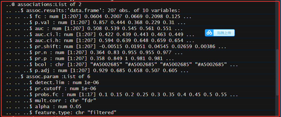
混杂因素可能导致关联检验的偏差。使用SIAMCAT来检验两个数据集(考虑丹麦样本和只考虑西班牙的样本)之间的关联。我们可以从SIAMCAT对象中提取关联指标,并将它们与散点图进行比较。
assoc.sp <- associations(sc.obj)
assoc.sp$species <- rownames(assoc.sp)
assoc.sp_dnk <- associations(sc.obj.full)
assoc.sp_dnk$species <- rownames(assoc.sp_dnk)

df.plot <- full_join(assoc.sp, assoc.sp_dnk, by='species')
df.plot %>%
    mutate(highlight=str_detect(species, 'formicigenerans')) %>%
    ggplot(aes(x=-log10(p.adj.x), y=-log10(p.adj.y), col=highlight)) +
    geom_point(alpha=0.3) +
        xlab('Spanish samples only\n-log10(q)') +
        ylab('Spanish and Danish samples only\n-log10(q)') +
        theme_classic() +
        theme(panel.grid.major = element_line(colour='lightgrey'),
            aspect.ratio = 1.3) +
        scale_colour_manual(values=c('darkgrey', '#D41645'), guide=FALSE) +
        annotate('text', x=0.7, y=8, label='Dorea formicigenerans')
结果发现,有几个物种,在考虑丹麦的健康对照样本时是显著的,但是只考虑西班牙的样本时是不显著的。例如*“Dorea formicigenerans”*。
# extract information out of the siamcat object
feat.dnk <- get.filt_feat.matrix(sc.obj.full)
label.dnk <- label(sc.obj.full)$label
country <- meta(sc.obj.full)$Country
names(country) <- rownames(meta(sc.obj.full))
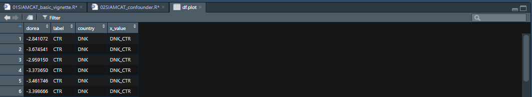
df.plot <- tibble(dorea=log10(feat.dnk[
str_detect(rownames(feat.dnk),'formicigenerans'),
names(label.dnk)] + 1e-05),
label=label.dnk, country=country) %>%
mutate(label=case_when(label=='-1'~'CTR', TRUE~"UC")) %>%
mutate(x_value=paste0(country, '_', label))
df.plot %>%
ggplot(aes(x=x_value, y=dorea)) +
geom_boxplot(outlier.shape = NA) +
geom_jitter(width = 0.08, stroke=0, alpha=0.2) +
theme_classic() +
xlab('') +
ylab("log10(Dorea formicigenerans)") +
stat_compare_means(comparisons = list(c('DNK_CTR', 'ESP_CTR'),
c('DNK_CTR', 'ESP_UC'),
c('ESP_CTR', 'ESP_UC')))
df.plot是一个291行,4列的DataFrame。
机器学习(Machine Learning):
机器学习工作流的结果也会受到国家之间的差异的影响,导致了夸大的性能估计。
sc.obj.full <- normalize.features(sc.obj.full, norm.method = 'log.std',
                                norm.param = list(log.n0=1e-06, sd.min.q=0))
## Features normalized successfully.
sc.obj.full <- create.data.split(sc.obj.full, num.folds = 5, num.resample = 5)
## Features splitted for cross-validation successfully.
sc.obj.full <- train.model(sc.obj.full, method='lasso')
## Trained lasso models successfully.
sc.obj.full <- make.predictions(sc.obj.full)
## Made predictions successfully.
sc.obj.full <- evaluate.predictions(sc.obj.full)
## Evaluated predictions successfully.
当我们比较两种不同模型的性能时,包含丹麦语和西班牙样本的模型似乎表现得更好(更高的AUROC值)。然而,之前的分析表明,这种性能估计是有偏见和夸大的,因为西班牙样本和丹麦样本之间的差异非常大。
model.evaluation.plot("Spanish samples only"=sc.obj,
                    "Danish and Spanish samples"=sc.obj.full,
                    fn.plot = './eval_plot_dnk.pdf')
## Plotted evaluation of predictions successfully to: ./eval_plot_dnk.pdf
为了演示机器学习模型如何利用这种混杂因素,我们可以训练一个模型来区分西班牙和丹麦的控制样本。 正如你所看到的,这个模型可以几乎完全准确地区分这两个国家。
meta.nielsen.country <- meta.nielsen[meta.nielsen$Group=='CTR',]

sc.obj.country <- siamcat(feat=feat, meta=meta.nielsen.country,
                            label='Country', case='ESP')
sc.obj.country <- filter.features(sc.obj.country, cutoff=1e-04,
                            filter.method = 'abundance')
sc.obj.country <- filter.features(sc.obj.country, cutoff=0.05,
                            filter.method='prevalence',
                            feature.type = 'filtered')
sc.obj.country <- normalize.features(sc.obj.country, norm.method = 'log.std',
                                    norm.param = list(log.n0=1e-06,
                                        sd.min.q=0))
sc.obj.country <- create.data.split(sc.obj.country,
                                    num.folds = 5, num.resample = 5)
sc.obj.country <- train.model(sc.obj.country, method='lasso')
sc.obj.country <- make.predictions(sc.obj.country)
sc.obj.country <- evaluate.predictions(sc.obj.country)

print(eval_data(sc.obj.country)$auroc)
## Area under the curve: 0.9701
值得参考的部分:
- 怎么对MetaPhlAn2和mOUTs2的输出进行预处理?进而将其导入
SIAMCAT对象,进行后续分析? - 怎么进行Confounder Analysis? 如何学习其图像的相关展示方法?
4.1.3 SIAMCAT holdout testing
参考:https://bioconductor.org/packages/release/bioc/vignettes/SIAMCAT/inst/doc/SIAMCAT_holdout.html
-
介绍( Introduction)
SIAMCAT包的功能之一是在宏基因组数据集上训练统计机器学习模型。本节教程,我们将展示一个数据集上训练的模型用于另一个独立的数据集(holdout dataset)。本节教程使用的两个结肠癌研究的数据集,第一个数据集来自法国( Zeller et al), 第二个数据集来自中国(Yu et al),连个数据集均使用mOTUs2预处理。 -
导入数据(Load the Data)
数据集可以从 Zeller group的公开宏基因组数据集网络资源找到。
library(SIAMCAT)

# this is data from Zeller et al., Mol. Syst. Biol. 2014
fn.feat.fr  <-
    'https://www.embl.de/download/zeller/FR-CRC/FR-CRC-N141_tax-ab-specI.tsv'
fn.meta.fr  <-
    'https://www.embl.de/download/zeller/FR-CRC/FR-CRC-N141_metadata.tsv'

# this is the external dataset from Yu et al., Gut 2017
fn.feat.cn  <-
    'https://www.embl.de/download/zeller/CN-CRC/CN-CRC-N128_tax-ab-specI.tsv'
fn.meta.cn  <-
    'https://www.embl.de/download/zeller/CN-CRC/CN-CRC-N128_metadata.tsv'
首先采用法国的项目,构建
SIAMCAT对象。# features # be vary of the defaults in R!!! feat.fr <- read.table(fn.feat.fr, sep='\t', quote="", check.names = FALSE, stringsAsFactors = FALSE) # the features are counts, but we want to work with relative abundances feat.fr.rel <- prop.table(as.matrix(feat.fr), 2) # metadata meta.fr <- read.table(fn.meta.fr, sep='\t', quote="", check.names=FALSE, stringsAsFactors=FALSE) # create SIAMCAT object siamcat.fr <- siamcat(feat=feat.fr.rel, meta=meta.fr, label='Group', case='CRC')然后加载中国研究,创建
SIAMCAT对象,作为holdout dataset。# features feat.cn <- read.table(fn.feat.cn, sep='\t', quote="", check.names = FALSE) feat.cn.rel <- prop.table(as.matrix(feat.cn), 2) # metadata meta.cn <- read.table(fn.meta.cn, sep='\t', quote="", check.names=FALSE, stringsAsFactors = FALSE) # SIAMCAT object siamcat.cn <- siamcat(feat=feat.cn.rel, meta=meta.cn, label='Group', case='CRC') -
在法国数据集上构建模型(Model Building on the French Dataset)
数据预处理(包括数据验证、过滤和标准化):
## 特征过滤
siamcat.fr <- filter.features(
    siamcat.fr,
    filter.method = 'abundance',
    cutoff = 0.001,
    rm.unmapped = TRUE,
    verbose=2
)

##特征标准化
siamcat.fr <- normalize.features(
    siamcat.fr,
    norm.method = "log.std",
    norm.param = list(log.n0 = 1e-06, sd.min.q = 0.1),
    verbose = 2
)
模型训练:
##交叉验证数据集划分
siamcat.fr <-  create.data.split(
    siamcat.fr,
    num.folds = 5,
    num.resample = 2
)

##训练模型
siamcat.fr <- train.model(
    siamcat.fr,
    method = "lasso"
)
预测, 在每个交叉验证折上进行预测,评估预测:
##进行预测 siamcat.fr <- make.predictions(siamcat.fr) ##评估预测 siamcat.fr <- evaluate.predictions(siamcat.fr) -
Application on the Holdout Dataset
现在,我们已经成功地为法国数据集构建了模型,我们可以将其应用到中国的holdout数据集。 首先,我们将使用与法国数据集相同的参数对中国数据集进行标准化,以使数据具有可比性。 对于这一步,我们可以在
SIAMCAT的normalize.features函数中使用冻结的标准化功能(frozen normalization functionality )。 我们为这个函数提供了保存在siamcat.fr对象中的所有标准化参数,其可以使用norm_params访问器访问这些参数。冻结标准化(Frozen Normalization):
##注意,标准化函数还是normalize.features,只是参数norm.param使用了法国数据集上的。
siamcat.cn <- normalize.features(siamcat.cn,
    norm.param=norm_params(siamcat.fr),
    feature.type='original',
    verbose = 2)
将训练的模型用于
holdout数据集。##使用siamcat.holdout参数来引入外部数据集。 siamcat.cn <- make.predictions( siamcat = siamcat.fr, siamcat.holdout = siamcat.cn, normalize.holdout = FALSE) ## Warning in make.predictions(siamcat = siamcat.fr, siamcat.holdout = ## siamcat.cn, : WARNING: holdout set is not being normalized!注意
make.predictions只能用于标准化以后的holdout数据集。## Alternative Code, not run here siamcat.cn <- siamcat(feat=feat.cn.rel, meta=meta.cn, label='Group', case='CRC') siamcat.cn <- make.predictions(siamcat = siamcat.fr, siamcat.holdout = siamcat.cn, normalize.holdout = TRUE)再次评估预测:
siamcat.cn <- evaluate.predictions(siamcat.cn) -
模型评估(Model Evaluation)
现在,我们可以使用
model.evaluation.plot比较原始分类器的性能和holdout数据集的性能。在这里,我们可以提供几个SIAMCAT对象,模型评估将被绘制在同一幅图中。 注意,我们可以以命名对象的形式提供对象,以便在图例中打印名称。model.evaluation.plot('FR-CRC'=siamcat.fr, 'CN-CRC'=siamcat.cn, colours=c('dimgrey', 'orange')
4.1.4 SIAMCAT input
参考: https://bioconductor.org/packages/release/bioc/vignettes/SIAMCAT/inst/doc/SIAMCAT_read-in.html
-
Introduction
本节教程将展示如何读取和输入你的数据到
SIAMCAT包。我们将覆盖从磁盘中读取文本文件、格式化数据并用它们来创建siamcat-class对象。siamcat-class是这个包的核心。所有输入维护局和结果都存储在里面。该对象的结构在下面的siamcat-class object部分描述。 -
Loading your data into R
整体而言,
SIAMCAT有三种类型的输入:特征(features), 元数据(Metadata)和标签(Label)。- features: 是
matrix, 或者data.frame, 或者otu_table,形式为features (in rows) x samples (in columns)。 - metadata: 应该是
matrix, 或者data.frame,形式为samples (in rows) x metadata (in columns)。 - label: Named vector, Metadata column,Label file。
library(SIAMCAT)
##读取特征表
fn.in.feat  <- system.file(
    "extdata",
    "feat_crc_zeller_msb_mocat_specI.tsv",
    package = "SIAMCAT"
)
feat <- read.table(fn.in.feat, sep='\t',
    header=TRUE, quote='',
    stringsAsFactors = FALSE, check.names = FALSE)
# look at some features
feat[110:114, 1:2]

##读取metadata表
fn.in.meta  <- system.file(
    "extdata",
    "num_metadata_crc_zeller_msb_mocat_specI.tsv",
    package = "SIAMCAT"
)
meta <- read.table(fn.in.meta, sep='\t',
    header=TRUE, quote='',
    stringsAsFactors = FALSE, check.names = FALSE)
head(meta)

##Finds the full file names of files in packages etc.
system.file(..., package = "base", lib.loc = NULL,
            mustWork = FALSE)
##...: character vectors, 指定某个包的特定子目录和文件。
##package: 指定单个包的名字。
##mustWork: 逻辑判断。 默认为TRUE,如果没有匹配的文件,返回错误。
指定标签:
label <- create.label(meta=meta, label="diagnosis",
    case = 1, control=0)

label <- create.label(meta=meta, label="diagnosis",
    case = 1, control=0,
    p.lab = 'cancer', n.lab = 'healthy')
当输入文件为lefse格式(biom-format)时,输入方法如下:
fn.in.lefse<- system.file(
    "extdata",
    "LEfSe_crc_zeller_msb_mocat_specI.tsv",
    package = "SIAMCAT"
)

##读取lefse文件
meta.and.features <- read.lefse(fn.in.lefse,
    rows.meta = 1:6, row.samples = 7)
meta <- meta.and.features$meta
feat <- meta.and.features$feat

##创建label
label <- create.label(meta=meta, label="label", case = "cancer")

##相关函数解析
##read an input file in a LEfSe input format
read.lefse(filename = "data.txt", rows.meta = 1, row.samples = 2)
##filename: LEfSe输入形式的输入文件名。
##row.meta: 指定哪些行存储的metadata变量。
##row.samples: 指定哪些行存储的是样本名称。
metagenomeSeq format files的输入文件:使用
read.table函数或者BIOM形式输入。BIOM format files:通过
phyloseq加入到SIAMCAT。文本文件首先通过phyloseq的import_biom导入。然后phyloseq对象可以被导入为siamcat对象。Creating a siamcat object of a phyloseq object:直接通过
siamcat构造函数,由phyloseq对象创建siamcat对象。data("GlobalPatterns") ## phyloseq example data label <- create.label(meta=sample_data(GlobalPatterns), label = "SampleType", case = c("Freshwater", "Freshwater (creek)", "Ocean")) # run the constructor function siamcat <- siamcat(phyloseq=GlobalPatterns, label=label) - features: 是
-
Creating a siamcat-class object
siamcat-class是整个包的核心。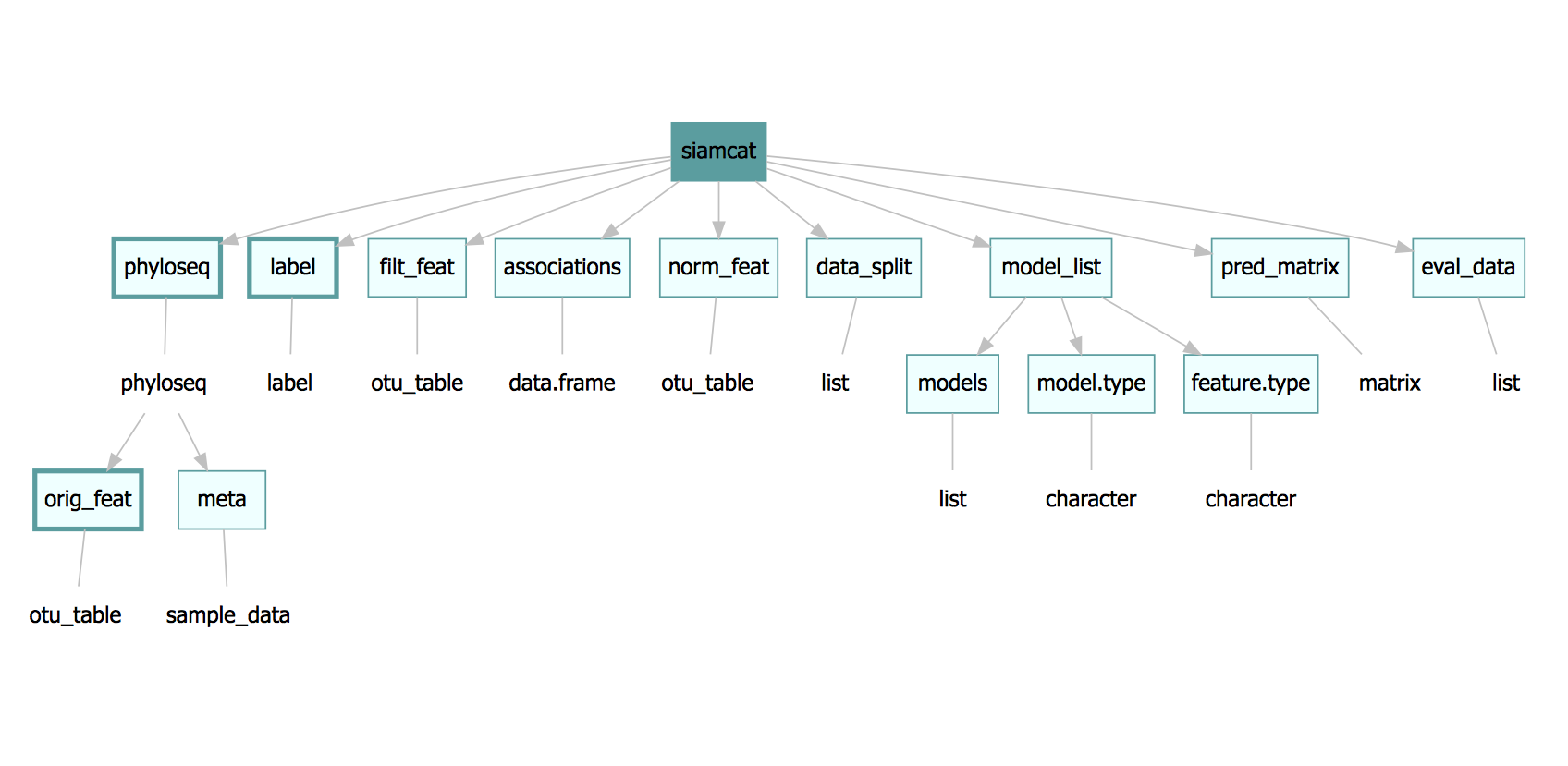
在上图中,矩形描述了对象的槽位,存储在槽位中的对象的类在椭圆中给出。有两个必须的槽位–phyloseq(包含作为
sample_data的metadata和作为otu_table的原始特征)以及label。这两个槽位用更粗的边框加以标识。siamcat对象的构建使用了siamcat函数,可以通过特征表Features或者phyloseq来初始化。siamcat <- siamcat(feat=feat, label=label, meta=meta) siamcat <- siamcat(phyloseq=phyloseq, label=label)-
phyloseq, label and orig_feat slots
help('phyloseq-class')
help('otu_table-class')
orig_feat(samcat.obj) ##可以使用orig_feat来获取siamcat对象的原始特征表。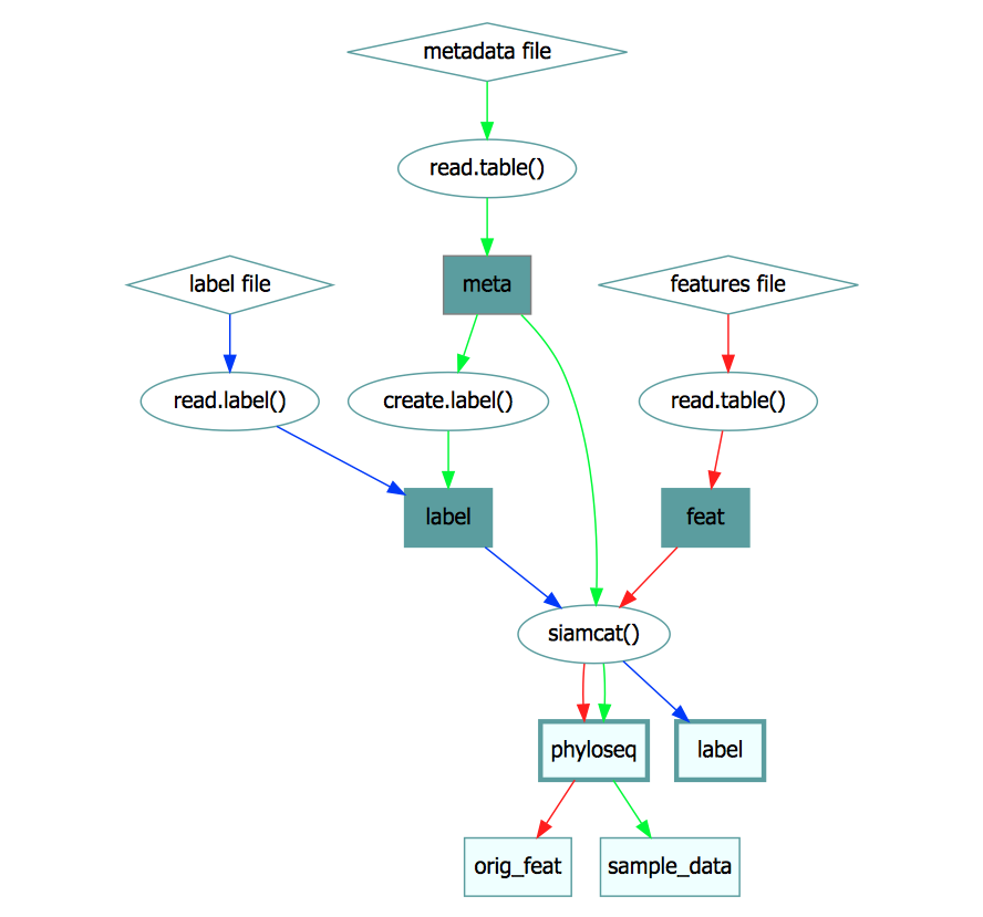
-
All the other slots
在运行
SIAMCAT的过程中,其他的卡槽也会被填充。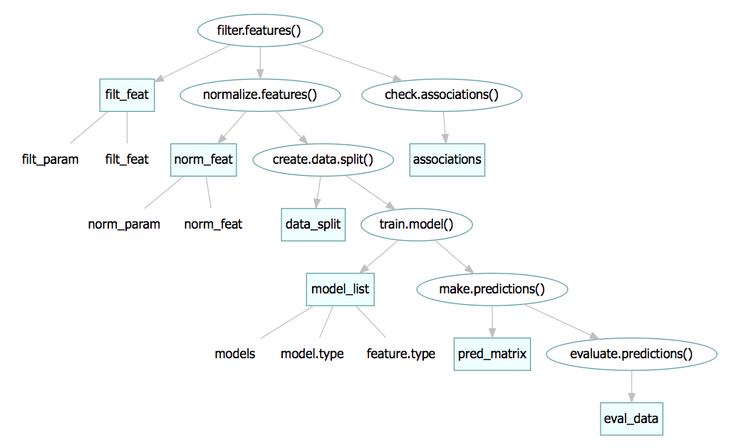
-
3. Accessing and assigning slots
siamcat中的每一个卡槽,都可以通过如下方式获取:
slot_name(siamcat)
例如,获取eval_data卡槽,你可以输入:
eval_data(siamcat)

##特例
physeq(siamcat)

##赋值
slot_name(siamcat) <- object_to_assign
label(siamcat) <- new_label
- Slots inside the slots
有两个插槽里面还有插槽。首先,model_list插槽中有models插槽,其包含了mlr模型的真实列表–能够通过models(siamcat)来获取。并且可以使用model.type()来获取训练模型的方法model_type(siamcat)。
phyloseq插槽有复杂的结构。然而,除非在SIAMCAT对象外面创建phyloseq对象,否则只有两个phyloseq插槽的插槽被占据:otu_table插槽包含着特征表,sam_data插槽包含metadata信息。分别可以通过features(siamcat)或者meta(siamcat)来获取。
phyloseq插槽中的其他插槽没有专门的访问器,但是从siamcat对象导出phyloseq对象后,很容易获取。
phyloseq <- physeq(siamcat)
tax_tab <- tax_table(phyloseq)
head(tax_tab)
如果你想要了解更多关于phyloseq数据结构的问题。可以查看phyloseq的BioConductor页面。
4.1.5 SIAMCAT meta-analysis
-
About This Vignette
本节教程,我们将展示
SIAMCAT如何促进宏基因组meta-analyses, 聚焦于关联测试和ML工作流程。作为案例,我们使用五个不同的**Crohn’s disease (CD)**研究,因为我们拥有来自5个不同数据集的宏基因组数据集。这些数据集是:开始(Setup)
library("tidyverse")
library("SIAMCAT")
首先,我们从所有研究中导入数据,其可以从EMBL的集群下载。原始数据经过预处理,然后使用 mOTUs2 来进行物种分类,然后聚焦genus水平。
# base url for data download
data.location <- 'https://www.embl.de/download/zeller/'
# datasets
datasets <- c('metaHIT', 'Lewis_2015', 'He_2017', 'Franzosa_2019', 'HMP2')
# metadata
meta.all <- read_tsv(paste0(data.location, 'CD_meta/meta_all.tsv'))
# features
feat <- read.table(paste0(data.location, 'CD_meta/feat_genus.tsv'),
                check.names = FALSE, stringsAsFactors = FALSE, quote = '',
                sep='\t')
feat <- as.matrix(feat)
# check that metadata and features agree
stopifnot(all(colnames(feat) == meta.all$Sample_ID))
让我们检查一下各个研究中分组的分布:
table(meta.all$Study, meta.all$Group) ## ## CD CTR ## Franzosa_2019 88 56 ## HMP2 583 357 ## He_2017 49 53 ## Lewis_2015 294 25 ## metaHIT 21 71某些研究可能包括来自同一受试者的多个样本。例如,HMP聚焦CD的纵向时间维度。因此,我们在训练和评估机器学习模型(查看Machine learning pitfalls部分的教程)以及进行关联分析时,要考虑这些问题。因此,为每个个体创建包含单个条目的第二个元数据表将很方便。
meta.ind <- meta.all %>% group_by(Individual_ID) %>% filter(Timepoint==min(Timepoint)) %>% ungroup() ##group_by(.data, ..., .add = FALSE, .drop = group_by_drop_default(.data)) 按照一个或多个变量来分组。 ##filter(.data, ..., .preserve = FALSE) 使用列名的值来对行取子集。 ##group_by(.data, ..., .add = FALSE, .drop = group_by_drop_default(.data)) 取消分组。 -
Compare Associations
使用SIAMCAT来计算关联。 为了检验关联,我们将每个数据集包裹为不同的
SIAMCAT对象,然后使用check.associations函数:assoc.list <- list() for (d in datasets){ # filter metadata and convert to dataframe meta.train <- meta.ind %>% filter(Study==d) %>% as.data.frame() rownames(meta.train) <- meta.train$Sample_ID # create SIAMCAT object sc.obj <- siamcat(feat=feat, meta=meta.train, label='Group', case='CD') # test for associations sc.obj <- check.associations(sc.obj, detect.lim = 1e-05, feature.type = 'original',fn.plot = paste0('./assoc_plot_', d, '.pdf')) # extract the associations and save them in the assoc.list temp <- associations(sc.obj) temp$genus <- rownames(temp) assoc.list[[d]] <- temp %>% select(genus, fc, auc, p.adj) %>% mutate(Study=d) } # combine all associations df.assoc <- bind_rows(assoc.list) df.assoc <- df.assoc %>% filter(genus!='unclassified') head(df.assoc) ## genus fc auc p.adj Study ## 159730 Thermovenabulum...1 159730 Thermovenabulum 0 0.5 NaN metaHIT ## 42447 Anaerobranca...2 42447 Anaerobranca 0 0.5 NaN metaHIT ## 1562 Desulfotomaculum...3 1562 Desulfotomaculum 0 0.5 NaN metaHIT ## 60919 Sanguibacter...4 60919 Sanguibacter 0 0.5 NaN metaHIT ## 357 Agrobacterium...5 357 Agrobacterium 0 0.5 NaN metaHIT ## 392332 Geoalkalibacter...6 392332 Geoalkalibacter 0 0.5 NaN metaHITPlot Heatmap for Interesting Genera. 比较存储在
df.assoc中的关联。例如,我们可以提取至少在一个数据集中与标签强烈相关的特征(single feature AUROC > 0.75 或 < 0.25),然后将the generalized fold change绘制为热图。genera.of.interest <- df.assoc %>% group_by(genus) %>% summarise(m=mean(auc), n.filt=any(auc < 0.25 | auc > 0.75), .groups='keep') %>% filter(n.filt) %>% arrange(m)提取了genera之后,我们绘制了它们:
df.assoc %>%
    # take only genera of interest
    filter(genus %in% genera.of.interest$genus) %>%
    # convert to factor to enforce an ordering by mean AUC
    mutate(genus=factor(genus, levels = rev(genera.of.interest$genus))) %>%
    # convert to factor to enforce ordering again
    mutate(Study=factor(Study, levels = datasets)) %>%
    # annotate the cells in the heatmap with stars
    mutate(l=case_when(p.adj < 0.01~'*', TRUE~'')) %>%
    ggplot(aes(y=genus, x=Study, fill=fc)) +
        geom_tile() +
        scale_fill_gradient2(low = '#3B6FB6', high='#D41645', mid = 'white',
            limits=c(-2.7, 2.7), name='Generalized\nfold change') +
        theme_minimal() +
        geom_text(aes(label=l)) +
        theme(panel.grid = element_blank()) +
        xlab('') + ylab('') +
        theme(axis.text = element_text(size=6))
反思:这种展示方式,可以用于NC-AD, NC-MCI, NC- SCS, NC-SCD种相关特征的比较。
-
Study as Confounding Factor
此外,我们还可以检查研究之间的差异是否会影响特定的genera的方差。为此,我们创建了单个
SIAMCAT对象,它拥有完整的数据集,然后运行check.confounder函数。df.meta <- meta.ind %>% as.data.frame() rownames(df.meta) <- df.meta$Sample_ID sc.obj <- siamcat(feat=feat, meta=df.meta, label='Group', case='CD') ## + starting create.label ## Label used as case: ## CD ## Label used as control: ## CTR ## + finished create.label.from.metadata in 0.001 s ## + starting validate.data ## +++ checking overlap between labels and features ## + Keeping labels of 504 sample(s). ## +++ checking sample number per class ## +++ checking overlap between samples and metadata ## + finished validate.data in 0.06 s check.confounders(sc.obj, fn.plot = './confounder_plot_cd_meta.pdf', feature.type='original') ## Finished checking metadata for confounders, results plotted to: ./confounder_plot_cd_meta.pdf结果方差图显示,某些generas受不同研究的影响很大,其他的genera则不是。 注意,随着标签信息(CD vs controls)变化很大的genera, 在不同的研究之间方差变化不是很大。
-
ML Meta-analysis
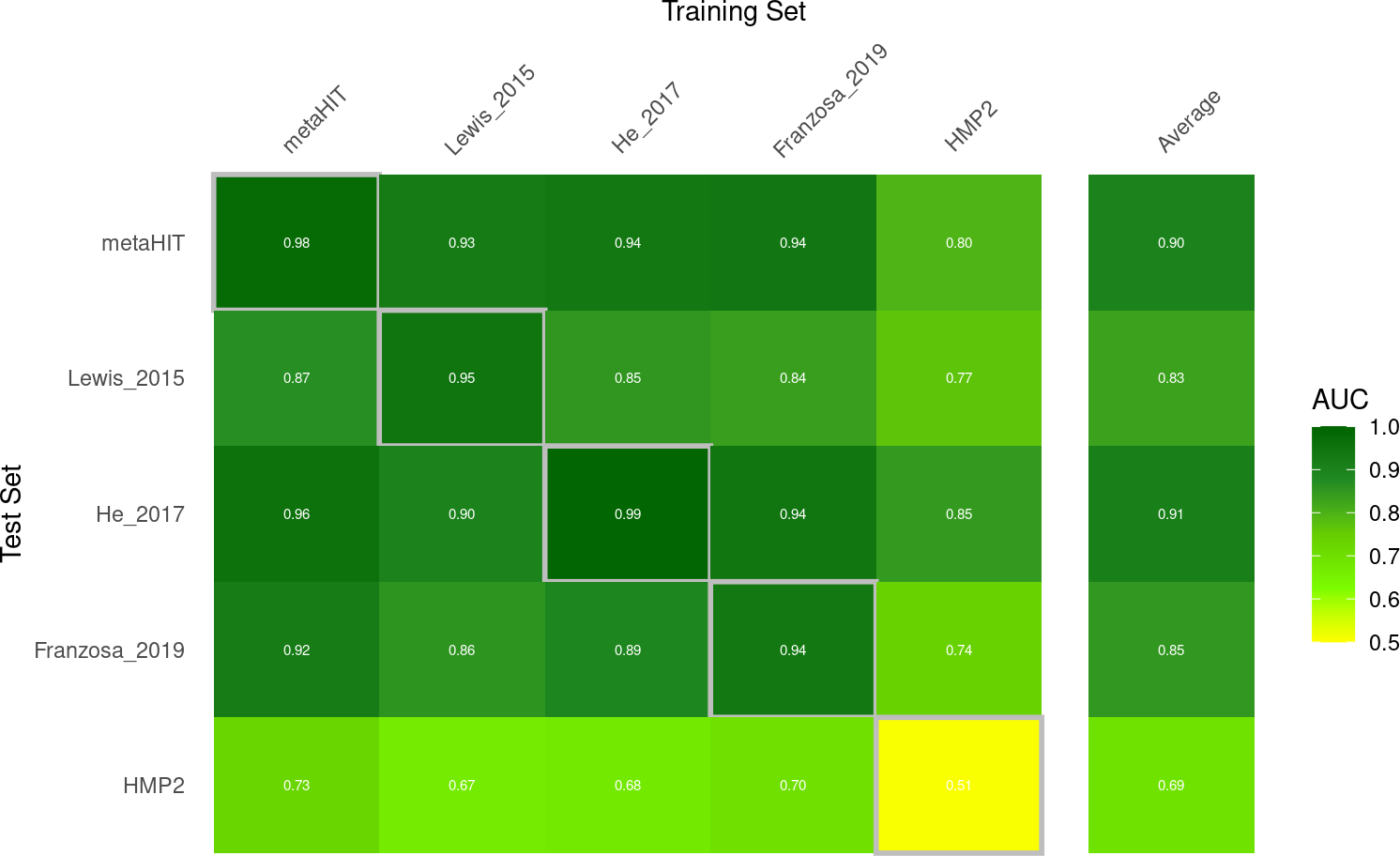
训练LASSO模型。最后,我们可以进行机器学习meta-analysis: 我们首先为每个数据集训练一个模型,然后使用SIAMCAT的holdout测试功能将其应用到其他数据集。对于跨受试者重复样本的数据集,我们阻止了受试者的交叉验证以避免结果偏差(参考Machine learning pitfalls)。
# create tibble to store all the predictions
auroc.all <- tibble(study.train=character(0),
                    study.test=character(0),
                    AUC=double(0))
# and a list to save the trained SIAMCAT objects
sc.list <- list()
for (i in datasets){
    # restrict to a single study
    meta.train <- meta.all %>%
        filter(Study==i) %>%
        as.data.frame()
    rownames(meta.train) <- meta.train$Sample_ID

    ## take into account repeated sampling by including a parameters
    ## in the create.data.split function
    ## For studies with repeated samples, we want to block the
    ## cross validation by the column 'Individual_ID'
    block <- NULL
    if (i %in% c('metaHIT', 'Lewis_2015', 'HMP2')){
        block <- 'Individual_ID'
        if (i == 'HMP2'){
            # for the HMP2 dataset, the number of repeated sample per subject
            # need to be reduced, because some subjects have been sampled
            # 20 times, other only 5 times
            meta.train <- meta.all %>%
                filter(Study=='HMP2') %>%
                group_by(Individual_ID) %>%
                sample_n(5, replace = TRUE) %>%
                distinct() %>%
                as.data.frame()
            rownames(meta.train) <- meta.train$Sample_ID
        }
    }
    # create SIAMCAT object
    sc.obj.train <- siamcat(feat=feat, meta=meta.train,
                            label='Group', case='CD')
    # normalize features
    sc.obj.train <- normalize.features(sc.obj.train, norm.method = 'log.std',
        norm.param=list(log.n0=1e-05, sd.min.q=0),feature.type = 'original')
    # Create data split
    sc.obj.train <- create.data.split(sc.obj.train,
        num.folds = 10, num.resample = 10, inseparable = block)
    # train LASSO model
    sc.obj.train <- train.model(sc.obj.train, method='lasso')

    ## apply trained models to other datasets

    # loop through datasets again
    for (i2 in datasets){
        if (i == i2){
            # make and evaluate cross-validation predictions (same dataset)
            sc.obj.train <- make.predictions(sc.obj.train)
            sc.obj.train <- evaluate.predictions(sc.obj.train)
            auroc.all <- auroc.all %>%
                add_row(study.train=i, study.test=i,
                    AUC=eval_data(sc.obj.train)$auroc %>% as.double())
        } else {
            # make and evaluate on the external datasets
            # use meta.ind here, since we want only one sample per subject!
            meta.test <- meta.ind %>%
                filter(Study==i2) %>%
                as.data.frame()
            rownames(meta.test) <- meta.test$Sample_ID
            sc.obj.test <- siamcat(feat=feat, meta=meta.test,
                                    label='Group', case='CD')
            # make holdout predictions
            sc.obj.test <- make.predictions(sc.obj.train,
                                            siamcat.holdout = sc.obj.test)
            sc.obj.test <- evaluate.predictions(sc.obj.test)
            auroc.all <- auroc.all %>%
                add_row(study.train=i, study.test=i2,
                    AUC=eval_data(sc.obj.test)$auroc %>% as.double())
        }
    }
    # save the trained model
    sc.list[[i]] <- sc.obj.train
}
训练了所有模型后,我们计算了每个数据集测试的平均。
test.average <- auroc.all %>%
    filter(study.train!=study.test) %>%
    group_by(study.test) %>%
    summarise(AUC=mean(AUC), .groups='drop') %>%
    mutate(study.train="Average")
现在,我们有了AUROC值,我们可以将它们绘制为很好的热图:
# combine AUROC values with test average
bind_rows(auroc.all, test.average) %>%
    # highlight cross validation versus transfer results
    mutate(CV=study.train == study.test) %>%
    # for facetting later
    mutate(split=case_when(study.train=='Average'~'Average', TRUE~'none')) %>%
    mutate(split=factor(split, levels = c('none', 'Average'))) %>%
    # convert to factor to enforce ordering
    mutate(study.train=factor(study.train, levels=c(datasets, 'Average'))) %>%
    mutate(study.test=factor(study.test, levels=c(rev(datasets),'Average'))) %>%
    ggplot(aes(y=study.test, x=study.train, fill=AUC, size=CV, color=CV)) +
        geom_tile() + theme_minimal() +
        # text in tiles
        geom_text(aes_string(label="format(AUC, digits=2)"),
            col='white', size=2)+
        # color scheme
        scale_fill_gradientn(colours=rev(c('darkgreen','forestgreen',
                                        'chartreuse3','lawngreen',
                                        'yellow')), limits=c(0.5, 1)) +
        # axis position/remove boxes/ticks/facet background/etc.
        scale_x_discrete(position='top') +
        theme(axis.line=element_blank(),
                axis.ticks = element_blank(),
                axis.text.x.top = element_text(angle=45, hjust=.1),
                panel.grid=element_blank(),
                panel.border=element_blank(),
                strip.background = element_blank(),
                strip.text = element_blank()) +
        xlab('Training Set') + ylab('Test Set') +
        scale_color_manual(values=c('#FFFFFF00', 'grey'), guide=FALSE) +
        scale_size_manual(values=c(0, 1), guide=FALSE) +
        facet_grid(~split, scales = 'free', space = 'free')
## Warning: It is deprecated to specify `guide = FALSE` to remove a guide. Please
## use `guide = "none"` instead.

## Warning: It is deprecated to specify `guide = FALSE` to remove a guide. Please
## use `guide = "none"` instead.
结果如下图所示:
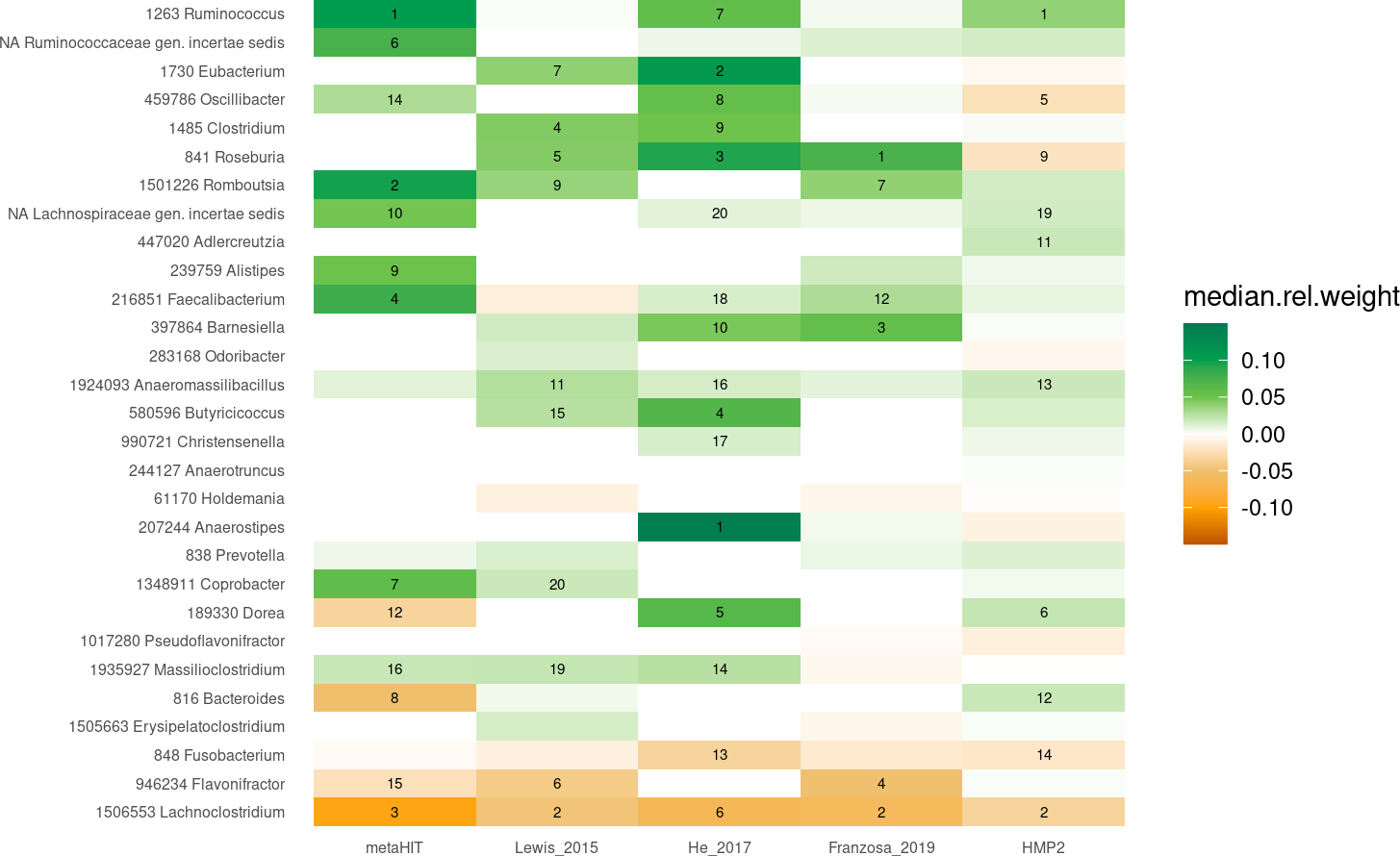
Investigate Feature Weights. 现在我们已经训练了模型(将其保存在sc.list对象中),我们可以使用SIAMCAT来提取模型的权重,比较我们上面计算的关联。
weight.list <- list()
for (d in datasets){
    sc.obj.train <- sc.list[[d]]
    # extract the feature weights out of the SIAMCAT object
    temp <- feature_weights(sc.obj.train)
    temp$genus <- rownames(temp)
    # save selected info in the weight.list
    weight.list[[d]] <- temp %>%
        select(genus, median.rel.weight, mean.rel.weight, percentage) %>%
        mutate(Study=d) %>%
        mutate(r.med=rank(-abs(median.rel.weight)),
            r.mean=rank(-abs(mean.rel.weight)))
}
# combine all feature weights into a single tibble
df.weights <- bind_rows(weight.list)
df.weights <- df.weights %>% filter(genus!='unclassified')
基于这个,我们可以绘制任何的热图,聚焦于我们在上面的关联热图中关注的genera。
# compute absolute feature weights
abs.weights <- df.weights %>%
    group_by(Study) %>%
    summarise(sum.median=sum(abs(median.rel.weight)),
                sum.mean=sum(abs(mean.rel.weight)),
                .groups='drop')

df.weights %>%
    full_join(abs.weights) %>%
    # normalize by the absolute model size
    mutate(median.rel.weight=median.rel.weight/sum.median) %>%
    # only include genera of interest
    filter(genus %in% genera.of.interest$genus) %>%
    # highlight feature rank for the top 20 features
    mutate(r.med=case_when(r.med > 20~NA_real_, TRUE~r.med)) %>%
    # enforce the correct ordering by converting to factors again
    mutate(genus=factor(genus, levels = rev(genera.of.interest$genus))) %>%
    mutate(Study=factor(Study, levels = datasets)) %>%
    ggplot(aes(y=genus, x=Study, fill=median.rel.weight)) +
        geom_tile() +
        scale_fill_gradientn(colours=rev(
            c('#007A53', '#009F4D', "#6CC24A", 'white',
            "#EFC06E", "#FFA300", '#BE5400')),
            limits=c(-0.15, 0.15)) +
        theme_minimal() +
        geom_text(aes(label=r.med), col='black', size= 2) +
        theme(panel.grid = element_blank()) +
        xlab('') + ylab('') +
        theme(axis.text = element_text(size=6))
## Joining, by = "Study"
4.1.6 SIAMCAT ML pitfalls
参考教程: https://www.bioconductor.org/packages/release/bioc/vignettes/SIAMCAT/inst/doc/SIAMCAT_ml_pitfalls.html
-
About This Vignette
在这个教程中,我们想要探索机器学习分析的两个陷阱,这可能会导致过于乐观的性能估计(过拟合,overfiting)。
在建立交叉验证工作流程时,通常是为了估计经过训练的模型在外部数据上的表现,这在考虑标记标记发现时是特别重要的。然而,更复杂的工作流涉及特征选择或时间序列数据(time-course data)可能对正确设置具有挑战性。从测试到测试数据的信息泄漏的错误工作流程,可能会导致过拟合,并且在外部数据集上泛化能力很糟糕。
在这里,我们关注的是监督特征选择和对依赖数据的简单划分。
Setup. 首先,我们加载分析所需的包。
如您所见,不正确的特征选择过程会导致 AUROC 值膨胀,但对真正外部数据集的泛化能力较低,尤其是在选择的特征很少时。 相反,正确的过程给出了较低的交叉验证结果,但可以更好地估计模型在外部数据上的表现。library("tidyverse") library("SIAMCAT") -
Supervised Feature Selection
监督式特征选择意味着在交叉验证划分之前就考虑标签信息。在该流程中,与标签相关的特征选择(例如差异丰度检验以后),使用整个数据集来计算特征关联,没有将数据放在一边来进行无偏的模型估计。
进行特征选择的正确方式是将特征选择步骤嵌入交叉验证步骤。这意味着在每个训练折中,特征关联的计算是独立进行的。
加载数据(Load the Data)。作为案例,我们将使用
curatedMetagenomicData包中的两个结肠癌(CRC)数据集。由于模型训练流程耗费很长的时间,这个教程没有在包的构建上进行评估,但是如果您为自己执行代码块,您应该得到类似的结果。library("curatedMetagenomicData")首先,我们加载Thomas et al的数据集作为训练集。
x <- 'ThomasAM_2018a.metaphlan_bugs_list.stool' feat.t <- curatedMetagenomicData(x=x, dryrun=FALSE) feat.t <- feat.t[[x]]@assayData$exprs # clean up metaphlan profiles to contain only species-level abundances feat.t <- feat.t[grep(x=rownames(feat.t), pattern='s__'),] feat.t <- feat.t[grep(x=rownames(feat.t),pattern='t__', invert = TRUE),] stopifnot(all(colSums(feat.t) != 0)) feat.t <- t(t(feat.t)/100)解决办法:R语言版本较低,需要升级为R4版本。https://www.cnblogs.com/chenwenyan/p/15064291.html
使用Zeller et al的数据集作为外部数据集:
x <- 'ZellerG_2014.metaphlan_bugs_list.stool'
feat.z <- curatedMetagenomicData(x=x, dryrun=FALSE)
feat.z <- feat.z[[x]]@assayData$exprs
# clean up metaphlan profiles to contain only species-level abundances
feat.z <- feat.z[grep(x=rownames(feat.z), pattern='s__'),]
feat.z <- feat.z[grep(x=rownames(feat.z),pattern='t__', invert = TRUE),]
stopifnot(all(colSums(feat.z) != 0))
feat.z <- t(t(feat.z)/100)
我们可以从
combined_metadata中提取对应的metadata信息,其是curatedMetagenomicData包的一部分。meta.t <- combined_metadata %>% filter(dataset_name == 'ThomasAM_2018a') %>% filter(study_condition %in% c('control', 'CRC')) rownames(meta.t) <- meta.t$sampleID meta.z <- combined_metadata %>% filter(dataset_name == 'ZellerG_2014') %>% filter(study_condition %in% c('control', 'CRC')) rownames(meta.z) <- meta.z$sampleIDMetaPhlAn2分类器的输出结果只展示数据集中出现的物种。因此,
ThomasAM_2018矩阵中包括的某些物种可能不包括在ZellerG_2014的矩阵中,或者相反。为了将它们作为SIAMCAT的训练集和外部测试集,我们首先要确定两个数据集中完全重叠的特征集合(可参看 Holdout Testing with SIAMCAT教程)。species.union <- union(rownames(feat.t), rownames(feat.z)) # add Zeller_2014-only species to the Thomas_2018 matrix add.species <- setdiff(species.union, rownames(feat.t)) feat.t <- rbind(feat.t, matrix(0, nrow=length(add.species), ncol=ncol(feat.t), dimnames = list(add.species, colnames(feat.t)))) # add Thomas_2018-only species to the Zeller_2014 matrix add.species <- setdiff(species.union, rownames(feat.z)) feat.z <- rbind(feat.z, matrix(0, nrow=length(add.species), ncol=ncol(feat.z), dimnames = list(add.species, colnames(feat.z)))) #注意相关函数现在,我们开始准备模型训练过程。对此,我们可以选择不同的特征选择阈值,准备一个tibble来保存结果。
fs.cutoff <- c(20, 100, 250)

auroc.all <- tibble(cutoff=character(0), type=character(0),
                    study.test=character(0), AUC=double(0))
首先,我们训练一个没有进行特征选择,有所有可用特征的模型。我们将
correct和incorrect的训练结果加入结果矩阵,用于后续绘图。sc.obj.t <- siamcat(feat=feat.t, meta=meta.t, label='study_condition', case='CRC') sc.obj.t <- filter.features(sc.obj.t, filter.method = 'prevalence', cutoff = 0.01) sc.obj.t <- normalize.features(sc.obj.t, norm.method = 'log.std', norm.param=list(log.n0=1e-05, sd.min.q=0)) sc.obj.t <- create.data.split(sc.obj.t, num.folds = 10, num.resample = 10) sc.obj.t <- train.model(sc.obj.t, method='lasso') sc.obj.t <- make.predictions(sc.obj.t) sc.obj.t <- evaluate.predictions(sc.obj.t) auroc.all <- auroc.all %>% add_row(cutoff='full', type='correct', study.test='Thomas_2018', AUC=as.numeric(sc.obj.t@eval_data$auroc)) %>% add_row(cutoff='full', type='incorrect', study.test='Thomas_2018', AUC=as.numeric(sc.obj.t@eval_data$auroc))接着,我们将模型用于外部数据集,记录其在另外一个数据集上的泛化能力。
sc.obj.z <- siamcat(feat=feat.z, meta=meta.z,
                    label='study_condition', case='CRC')
sc.obj.z <- make.predictions(sc.obj.t, sc.obj.z)
sc.obj.z <- evaluate.predictions(sc.obj.z)
auroc.all <- auroc.all %>%
    add_row(cutoff='full', type='correct',
            study.test='Zeller_2014',
            AUC=as.numeric(sc.obj.z@eval_data$auroc)) %>%
    add_row(cutoff='full', type='incorrect',
            study.test='Zeller_2014',
            AUC=as.numeric(sc.obj.z@eval_data$auroc))
**错误的流程:基于监督式特征选择的训练。**在不正确的特征选择流程中,我们使用整个数据集,基于差异风度检测了特征,然后选择高度相关的特征。
sc.obj.t <- check.associations(sc.obj.t, detect.lim = 1e-05,
                                fn.plot = 'assoc_plot.pdf')
mat.assoc <- associations(sc.obj.t)
mat.assoc$species <- rownames(mat.assoc)
# sort by p-value
mat.assoc <- mat.assoc %>% as_tibble() %>% arrange(p.val)
基于
check.association函数的P values, 我们选择X个特征用于训练模型。for (x in fs.cutoff){ # select x number of features based on p-value ranking feat.train.red <- feat.t[mat.assoc %>% slice(seq_len(x)) %>% pull(species),] sc.obj.t.fs <- siamcat(feat=feat.train.red, meta=meta.t, label='study_condition', case='CRC') # normalize the features without filtering sc.obj.t.fs <- normalize.features(sc.obj.t.fs, norm.method = 'log.std', norm.param=list(log.n0=1e-05,sd.min.q=0),feature.type = 'original') # take the same cross validation split as before data_split(sc.obj.t.fs) <- data_split(sc.obj.t) # train sc.obj.t.fs <- train.model(sc.obj.t.fs, method = 'lasso') # make predictions sc.obj.t.fs <- make.predictions(sc.obj.t.fs) # evaluate predictions and record the result sc.obj.t.fs <- evaluate.predictions(sc.obj.t.fs) auroc.all <- auroc.all %>% add_row(cutoff=as.character(x), type='incorrect', study.test='Thomas_2018', AUC=as.numeric(sc.obj.t.fs@eval_data$auroc)) # apply to the external dataset and record the result sc.obj.z <- siamcat(feat=feat.z, meta=meta.z, label='study_condition', case='CRC') sc.obj.z <- make.predictions(sc.obj.t.fs, sc.obj.z) sc.obj.z <- evaluate.predictions(sc.obj.z) auroc.all <- auroc.all %>% add_row(cutoff=as.character(x), type='incorrect', study.test='Zeller_2014', AUC=as.numeric(sc.obj.z@eval_data$auroc)) }正确的流程: 嵌套特征选择的训练。 将特征选择嵌套到交叉验证流程中,是特征选择的正确方式。我们通过指定
SIAMCAT包中的train.model函数的perform.fs参数,可以实现嵌套交叉验证流程。for (x in fs.cutoff){ # train using the original SIAMCAT object # with correct version of feature selection sc.obj.t.fs <- train.model(sc.obj.t, method = 'lasso', perform.fs = TRUE, param.fs = list(thres.fs = x,method.fs = "AUC",direction='absolute')) # make predictions sc.obj.t.fs <- make.predictions(sc.obj.t.fs) # evaluate predictions and record the result sc.obj.t.fs <- evaluate.predictions(sc.obj.t.fs) auroc.all <- auroc.all %>% add_row(cutoff=as.character(x), type='correct', study.test='Thomas_2018', AUC=as.numeric(sc.obj.t.fs@eval_data$auroc)) # apply to the external dataset and record the result sc.obj.z <- siamcat(feat=feat.z, meta=meta.z, label='study_condition', case='CRC') sc.obj.z <- make.predictions(sc.obj.t.fs, sc.obj.z) sc.obj.z <- evaluate.predictions(sc.obj.z) auroc.all <- auroc.all %>% add_row(cutoff=as.character(x), type='correct', study.test='Zeller_2014', AUC=as.numeric(sc.obj.z@eval_data$auroc)) }**结果绘图。**现在,我们来绘制结果性能图,来评估交叉验证和外部验证的性能。
auroc.all %>%
    # facetting for plotting
    mutate(split=case_when(study.test=="Thomas_2018"~
                            'Cross validation (Thomas 2018)',
                        TRUE~"External validation (Zeller 2014)")) %>%
    # convert to factor to enforce ordering
    mutate(cutoff=factor(cutoff, levels = c(fs.cutoff, 'full'))) %>%
    ggplot(aes(x=cutoff, y=AUC, col=type)) +
        geom_point() + geom_line(aes(group=type)) +
        facet_grid(~split) +
        scale_y_continuous(limits = c(0.5, 1), expand = c(0,0)) +
        xlab('Features selected') +
        ylab('AUROC') +
        theme_bw() +
        scale_colour_manual(values = c('correct'='blue', 'incorrect'='red'),
            name='Feature selection procedure') +
        theme(panel.grid.minor = element_blank(), legend.position = 'bottom')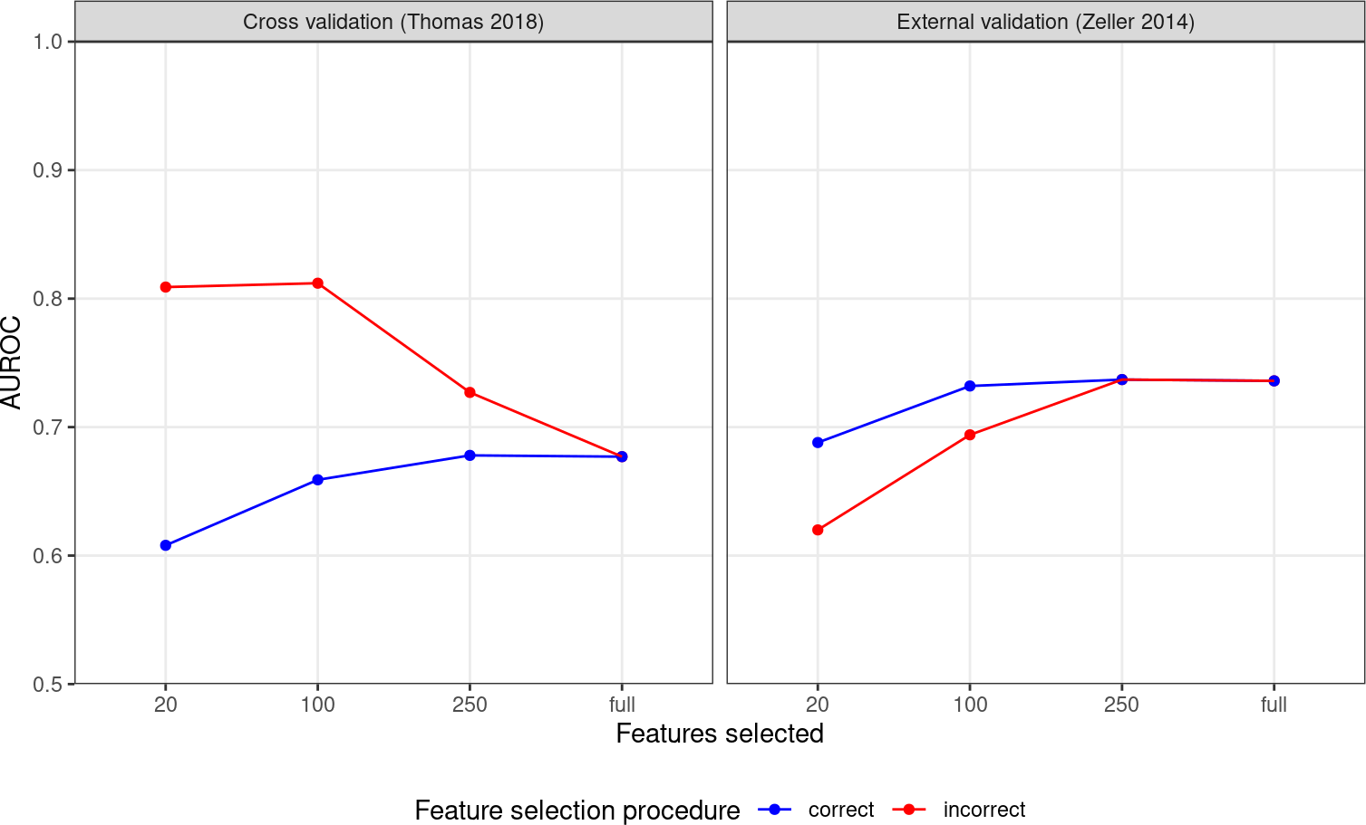
如您所见,不正确的特征选择过程会导致 AUROC 值膨胀,但对真正外部数据集的泛化能力较低,尤其是在选择的特征很少时。 相反,正确的过程给出了较低的交叉验证结果,但可以更好地估计模型在外部数据上的表现。
-
Naive Splitting of Dependent Data
当样本不独立时,机器学习工作流程中可能会出现另一个问题。 例如,在不同时间点从同一个体采集的微生物组样本通常比从其他个体采集的样本更相似。 如果这些样本在简单的交叉验证过程中被随机拆分,则可能会出现来自同一个人的样本最终会出现在训练和测试折叠(fold)中的情况。 在这种情况下,与应该学习区分个体标签的期望模型相比,该模型将学习对同一个体的跨时间点进行泛化。为避免此问题,需要在交叉验证期间阻止相关测量,以确保同一块内的样本将保持在同一折叠中(用于训练和测试)。
**加载数据。**我们使用EMBL集群上的多个Crohn’s disease (CD) 数据集作为案例。该数据集已经进行了过滤和清洗。由于模型训练要花费很长的时间,所以这部分教程没有实际执行,你可以尝试自己执行它。
data.location <- 'https://www.embl.de/download/zeller/'

# metadata
meta.all <- read_tsv(paste0(data.location, 'CD_meta/meta_all.tsv'))
## Rows: 1597 Columns: 6
## ── Column specification ────────────────────────────────────────────────────────
## Delimiter: "\t"
## chr (4): Sample_ID, Group, Individual_ID, Study
## dbl (2): Library_Size, Timepoint
##
## ℹ Use `spec()` to retrieve the full column specification for this data.
## ℹ Specify the column types or set `show_col_types = FALSE` to quiet this message.

# features
feat.motus <- read.table(paste0(data.location, 'CD_meta/feat_rel_filt.tsv'),
                        sep='\t', stringsAsFactors = FALSE,
                        check.names = FALSE)
当我们检查样本数目和受试者数目时,我们发现
HMP研究中存在某个受试者对应多个样本的情况。x <- meta.all %>% group_by(Study, Group) %>% summarise(n.all=n(), .groups='drop') y <- meta.all %>% select(Study, Group, Individual_ID) %>% distinct() %>% group_by(Study, Group) %>% summarize(n.indi=n(), .groups='drop') full_join(x,y) ## Joining, by = c("Study", "Group") ## # A tibble: 10 × 4 ## Study Group n.all n.indi ## <chr> <chr> <int> <int> ## 1 Franzosa_2019 CD 88 88 ## 2 Franzosa_2019 CTR 56 56 ## 3 HMP2 CD 583 50 ## 4 HMP2 CTR 357 26 ## 5 He_2017 CD 49 49 ## 6 He_2017 CTR 53 53 ## 7 Lewis_2015 CD 294 85 ## 8 Lewis_2015 CTR 25 25 ## 9 metaHIT CD 21 13 ## 10 metaHIT CTR 71 59因此,我们将在
HMP2训练模型。但是每个受试者的样本数目变化很大,因此我们希望在每个受试者上随机选择5个样本。【问题:为什么每个受试者可以选5个样本呢?选了5个样本之后,如何正确进行测试和交叉验证?】meta.all %>% filter(Study=='HMP2') %>% group_by(Individual_ID) %>% summarise(n=n(), .groups='drop') %>% pull(n) %>% hist(20)# sample 5 samples per individual meta.train <- meta.all %>% filter(Study=='HMP2') %>% group_by(Individual_ID) %>% sample_n(5, replace = TRUE) %>% distinct() %>% as.data.frame() rownames(meta.train) <- meta.train$Sample_ID对于评估,我们只想每个受试者只选一个样本,因此我们创建了新的矩阵,来去掉其他研究中重复的样本。
meta.ind <- meta.all %>%
    group_by(Individual_ID) %>%
    filter(Timepoint==min(Timepoint)) %>%
    ungroup()
最后,我们准备创建一个tibble来存储所有的AUROC值。
auroc.all <- tibble(type=character(0), study.test=character(0), AUC=double(0))基于朴素交叉验证的训练(Train with Naive Cross-validation)。 朴素交叉验证的样本划分不考虑样本间的依赖性。因此,大致流程如下所示:
sc.obj <- siamcat(feat=feat.motus, meta=meta.train,
                    label='Group', case='CD')
sc.obj <- normalize.features(sc.obj, norm.method = 'log.std',
    norm.param=list(log.n0=1e-05,sd.min.q=1),feature.type = 'original')
sc.obj.naive <- create.data.split(sc.obj, num.folds = 10, num.resample = 10)
sc.obj.naive <- train.model(sc.obj.naive, method='lasso')
sc.obj.naive <- make.predictions(sc.obj.naive)
sc.obj.naive <- evaluate.predictions(sc.obj.naive)
auroc.all <- auroc.all %>%
    add_row(type='naive', study.test='HMP2',
        AUC=as.numeric(eval_data(sc.obj.naive)$auroc))
**基于阻塞交叉验证的训练(Train with Blocked Cross-validation)。**正确的方式要考虑来自同一受试者的重复样本,进行阻塞式的交叉验证。这种方式下,来自同一受试者的样本将始终在同一个折中结束。这可以通过指定
SIAMCAT包中create.data.split函数的inseparable参数来实现。sc.obj.block <- create.data.split(sc.obj, num.folds = 10, num.resample = 10, inseparable = 'Individual_ID') sc.obj.block <- train.model(sc.obj.block, method='lasso') sc.obj.block <- make.predictions(sc.obj.block) sc.obj.block <- evaluate.predictions(sc.obj.block) auroc.all <- auroc.all %>% add_row(type='blocked', study.test='HMP2', AUC=as.numeric(eval_data(sc.obj.block)$auroc)) ##Split a dataset into training and a test sets. ##create.data.split(siamcat, num.folds = 2, num.resample = 1, stratify = TRUE, inseparable = NULL, verbose = 1) ##如果提供了inseparable参数,数据拆分将考虑用于数据拆分的metadata avaiable. 例如,数据包括来自同一个受试者的多个样本,在同一折中保留来自同一个人的数据是有意义的。如果给出了inseparable参数,将忽略stratify参数。**用于外部数据集(Apply to External Datasets)。**现在我们可以将模型用于外部数据集,并记录结果准确率。
Plot the Resultsfor (i in setdiff(unique(meta.all$Study), 'HMP2')){
    meta.test <- meta.ind %>%
        filter(Study==i) %>%
        as.data.frame()
    rownames(meta.test) <- meta.test$Sample_ID
    # apply naive model
    sc.obj.test <- siamcat(feat=feat.motus, meta=meta.test,
                            label='Group', case='CD')
    sc.obj.test <- make.predictions(sc.obj.naive, sc.obj.test)
    sc.obj.test <- evaluate.predictions(sc.obj.test)
    auroc.all <- auroc.all %>%
    add_row(type='naive', study.test=i,
            AUC=as.numeric(eval_data(sc.obj.test)$auroc))
    # apply blocked model
    sc.obj.test <- siamcat(feat=feat.motus, meta=meta.test,
                            label='Group', case='CD')
    sc.obj.test <- make.predictions(sc.obj.block, sc.obj.test)
    sc.obj.test <- evaluate.predictions(sc.obj.test)
    auroc.all <- auroc.all %>%
        add_row(type='blocked', study.test=i,
                AUC=as.numeric(eval_data(sc.obj.test)$auroc))
}
**绘制结果(Plot the Results)。**现在我们比较两种不同的方法得到的AUROC值。
auroc.all %>%
    # convert to factor to enforce ordering
    mutate(type=factor(type, levels = c('naive', 'blocked'))) %>%
    # facetting for plotting
    mutate(CV=case_when(study.test=='HMP2'~'CV',
                        TRUE~'External validation')) %>%
    ggplot(aes(x=study.test, y=AUC, fill=type)) +
        geom_bar(stat='identity', position = position_dodge(), col='black') +
        theme_bw() +
        coord_cartesian(ylim=c(0.5, 1)) +
        scale_fill_manual(values=c('red', 'blue'), name='') +
        facet_grid(~CV, space = 'free', scales = 'free') +
        xlab('') + ylab('AUROC') +
        theme(legend.position = c(0.8, 0.8))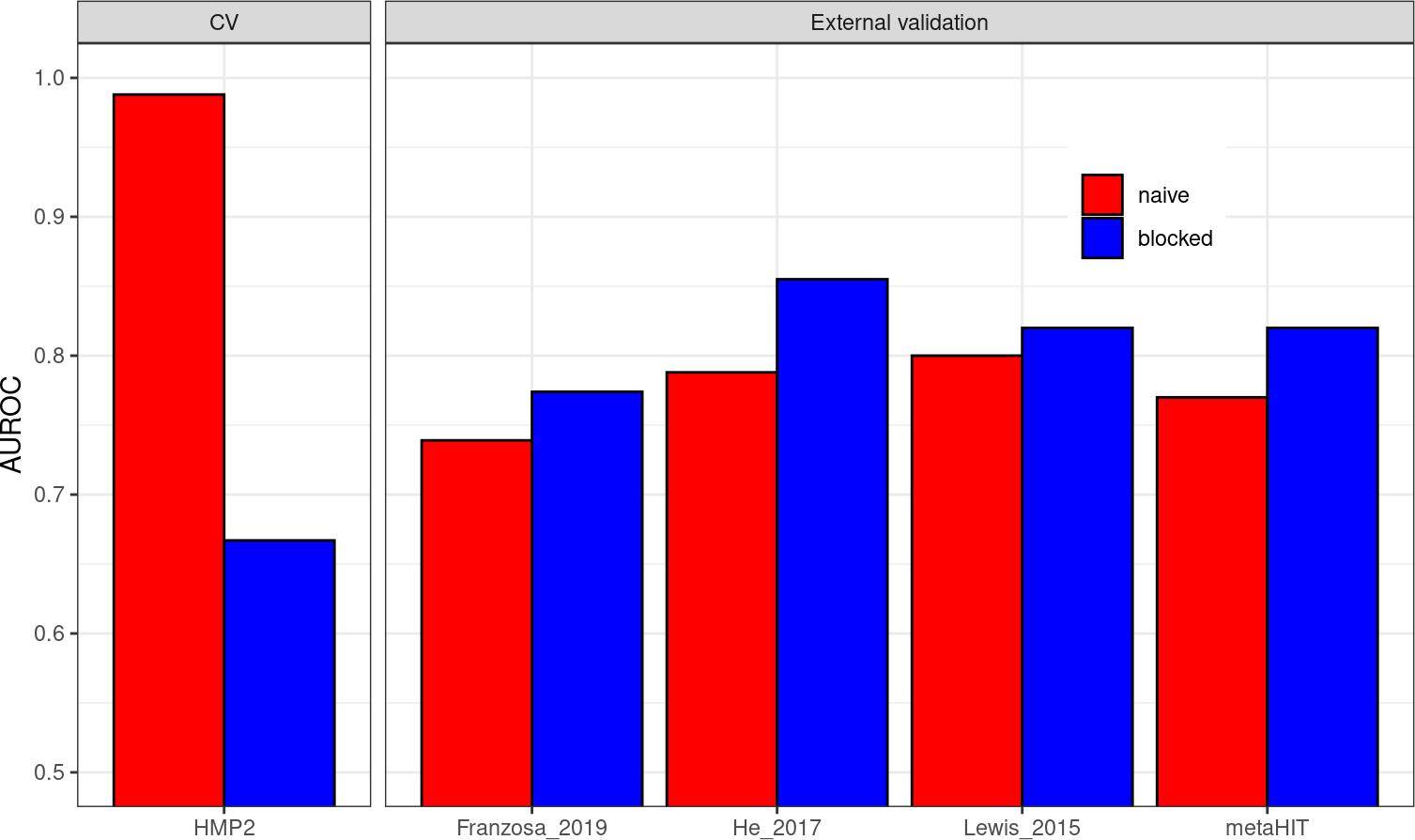
如你所见,朴素的交叉验证流程相比阻塞交叉验证导致了性能的膨胀。然而,当评估外部数据集的泛化性能时,阻塞交叉验证流程导致了更好的性能。


 642
642

 被折叠的 条评论
为什么被折叠?
被折叠的 条评论
为什么被折叠?
 到【灌水乐园】发言


