吴恩达Deep Learning编程作业 Course2- 改善深层神经网络：超参数调试、 正则化以及优化-第一周作业

吴恩达Deep Learning编程作业 Course2- 改善深层神经网络：超参数调试、 正则化以及优化-第一周作业

初始化、正则化、梯度校验

1.初始化

这一部分我们将学习如何为一个初始的神经网络设置初始化参数，不同的初始化方式会产生不同的效果，现在我们就一起来尝试。

首先我们先来了解一下什么样的初始化方法是好的方法：

• 加速梯度下降的收敛
• 增加梯度下降收敛到较低的训练(和泛化)错误的几率

1.1 加载数据

代码：

def load_dataset():
    np.random.seed(1)
    train_X, train_Y = sklearn.datasets.make_circles(n_samples=300, noise=.05)
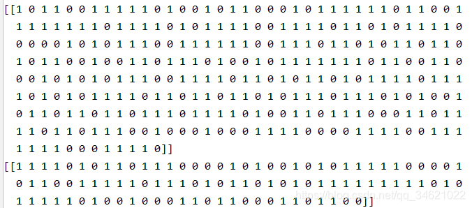
    print(train_X.shape)
    print(train_Y.shape)
    np.random.seed(2)
    #train_X.shape=(300,2) train_Y.shape=(300,)
    test_X, test_Y = sklearn.datasets.make_circles(n_samples=100, noise=.05)
    # Visualize the data
    plt.scatter(train_X[:, 0], train_X[:, 1], c=train_Y, s=40, cmap=plt.cm.Spectral);
    train_X = train_X.T
    train_Y = train_Y.reshape((1, train_Y.shape[0]))
    test_X = test_X.T
    test_Y = test_Y.reshape((1, test_Y.shape[0]))
    return train_X, train_Y, test_X, test_Y

调用：

import numpy as np
import matplotlib.pyplot as plt
import sklearn
import sklearn.datasets
from Week2.Utils.init_utils import load_dataset, forward_propagation, compute_loss, backward_propagation, \
    update_parameters, predict, predict_dec, plot_decision_boundary

#设置画布属性
plt.rcParams['figure.figsize'] = (7.0, 4.0)
plt.rcParams['image.interpolation'] = 'nearest'
plt.rcParams['image.cmap'] = 'gray'

if __name__ == '__main__':
    #加载数据
    train_X, train_Y, test_X, test_Y = load_dataset()

运行结果：

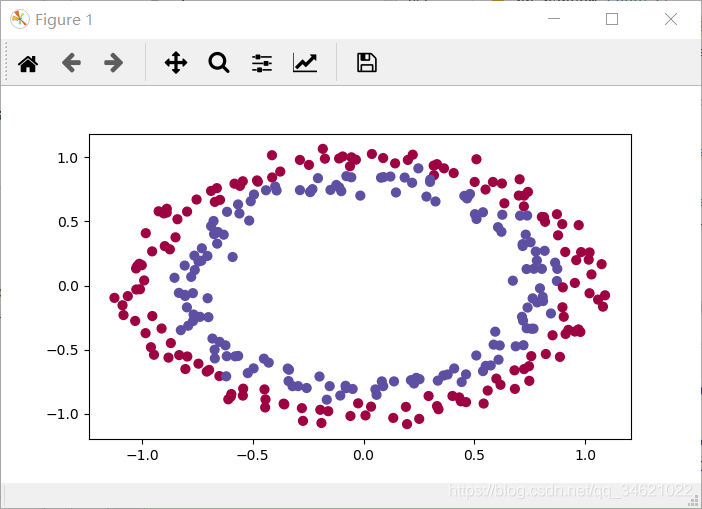
注意为了方便公式的计算，我们一般把读取出来的数据的维数设置为：
X：（特征数，数据量）；Y：（输出单元个数–一般为1，数据量）
可以结合公式$Z=W^{T}X+b$理解。

1.2 神经网络模型的参数初始化

下面我们将为一个三层的神经网络模型初始化参数，我们进行实验的方法一共有三种：

• 零初始化：将所有的参数设置为0
• 随机初始化：将权重设置为较大的随机数。
• He初始化：根据He等人2015年的一篇论文，该方法将权重初始化为随机值。

接下来我们先实现一个三层的神经网络模型，用于实验三种初始化方式。
代码：

def model(X, Y, learning_rate=0.01, num_iterations=15000, print_cost=True, initialization="he"):
    """
    实现了一个三层的神经网络:LINEAR->RELU->LINEAR->RELU->LINEAR->SIGMOID
    :param X:输入的数据，shape（2，300）
    :param Y:数据标签（1，300）
    :param learning_rate:学习率
    :param num_iterations:迭代次数
    :param print_cost:是否每100次打印代价
    :param initialization:初始化方式
    :return:返回学习到的参数
    """
    grads = ()
    costs = []
    m = X.shape[1]
    layers_dims = [X.shape[0], 10, 5, 1]

    if initialization == "zeros":
        parameters = initialize_parameters_zeros(layers_dims)
    elif initialization == "random":
        parameters = initialize_parameters_random(layers_dims)
    elif initialization == "he":
        parameters = initialize_parameters_he(layers_dims)

    for i in range(0, num_iterations):
        #1.前向传播
        a3, cache = forward_propagation(X, parameters)
        #2.计算代价
        cost = compute_loss(a3, Y)
        #3.反向传播
        grads = backward_propagation(X, Y, cache)
        #4.更新参数
        parameters = update_parameters(parameters, grads, learning_rate)

        if print_cost and i % 1000 == 0:
            print("Cost after iteration {}: {}".format(i, cost))
            costs.append(cost)

        # plot the loss
        plt.plot()
        plt.plot(costs)
        plt.ylabel('cost')
        plt.xlabel('iterations (per hundreds)')
        plt.title("Learning rate =" + str(learning_rate))
        plt.show()

1.21 初始化参数为0

需要初始化的参数有
1.权重矩阵$(W^{[1]},W^{[2]},W^{[3]},...,W^{[L-1]},W^{[L]})$
2.偏置矩阵$(b^{[1]},b^{[2]},b^{[3]},...,b^{[L-1]},b^{[L]})$
代码：

def initialize_parameters_zeros(layer_dims):
    parameters = {}
    L = len(layer_dims)
    for l in range(1, L):
        parameters['W' + str(l)] = np.zeros((layer_dims[l], layer_dims[l-1]))
        parameters['b' + str(l)] = np.zeros((layer_dims[l], 1))

    return parameters

调用：

parameters = initialize_parameters_zeros([3, 2, 1])
    print("W1 = " + str(parameters["W1"]))
    print("b1 = " + str(parameters["b1"]))
    print("W2 = " + str(parameters["W2"]))
    print("b2 = " + str(parameters["b2"]))

运行结果：

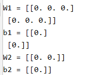
看一下使用这种方法初始化参数后运行的结果：
代码：

 train_X, train_Y, test_X, test_Y = load_dataset()
    parameters = initialize_parameters_zeros([3, 2, 1])
    print("W1 = " + str(parameters["W1"]))
    print("b1 = " + str(parameters["b1"]))
    print("W2 = " + str(parameters["W2"]))
    print("b2 = " + str(parameters["b2"]))

    parameters = model(train_X, train_Y, initialization="zeros")
    print("On the train set:")
    predictions_train = predict(train_X, train_Y, parameters)
    print("On the test set:")
    predictions_test = predict(test_X, test_Y, parameters)

运行结果：

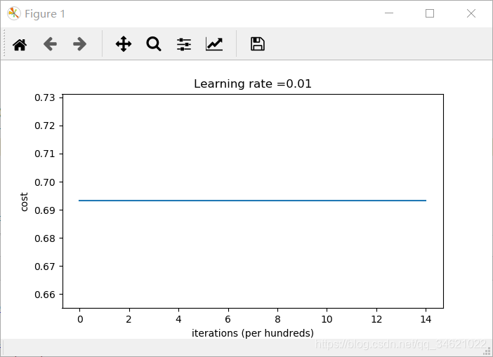
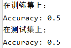
从准确率来看，得到的预测值和随机预测一样.
模型对每个例子都预测为0。通常，将所有的权值初始化为0会导致网络无法打破对称性。这意味着每一层中的每个神经元都将学习相同的内容，我们还可以训练一个每一层$n^{[l]}=1$的神经网络，而该网络并不比逻辑回归等线性分类器更强大。权值$W^{[l]}$应该被随机初始化以打破对称性。但是，可以将偏差$b^{[l]}$初始化为零。只要$W^{[l]}$被随机初始化，对称仍然是不对称的。

1.22 随机初始化

为了打破对称性，我们随机初始化权值。在随机初始化之后，每个神经元可以继续学习其输入的不同函数。在这个练习中，我们将看到如果权重是随机初始化的，但是是非常大的值，会发生什么。
代码：

def initialize_parameters_random(layer_dims):
    #这句话是为了你和我得到一样的结果，真正写模型用到随机生成时不需要写
    np.random.seed(3)
    parameters = {}
    L = len(layer_dims)

    for l in range(1, L):
        parameters['W' + str(l)] = np.random.randn(layer_dims[l], layer_dims[l - 1]) * 10
        parameters['b' + str(l)] = np.zeros((layer_dims[l], 1))

    return parameters

调用：

    parameters = initialize_parameters_random([3, 2, 1])
    print("W1 = " + str(parameters["W1"]))
    print("b1 = " + str(parameters["b1"]))
    print("W2 = " + str(parameters["W2"]))
    print("b2 = " + str(parameters["b2"]))

结果：

运用到三层神经网络模型中：
代码：

    parameters = model(train_X, train_Y, initialization="random")
    print("On the train set:")
    predictions_train = predict(train_X, train_Y, parameters)
    print("On the test set:")
    predictions_test = predict(test_X, test_Y, parameters)

运行结果：


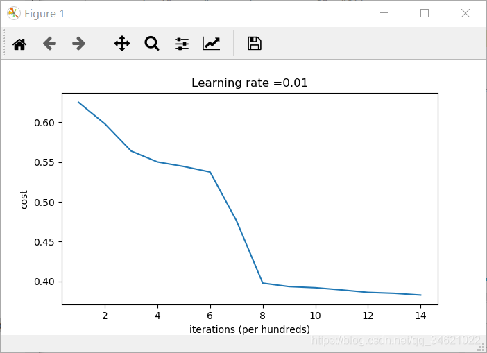
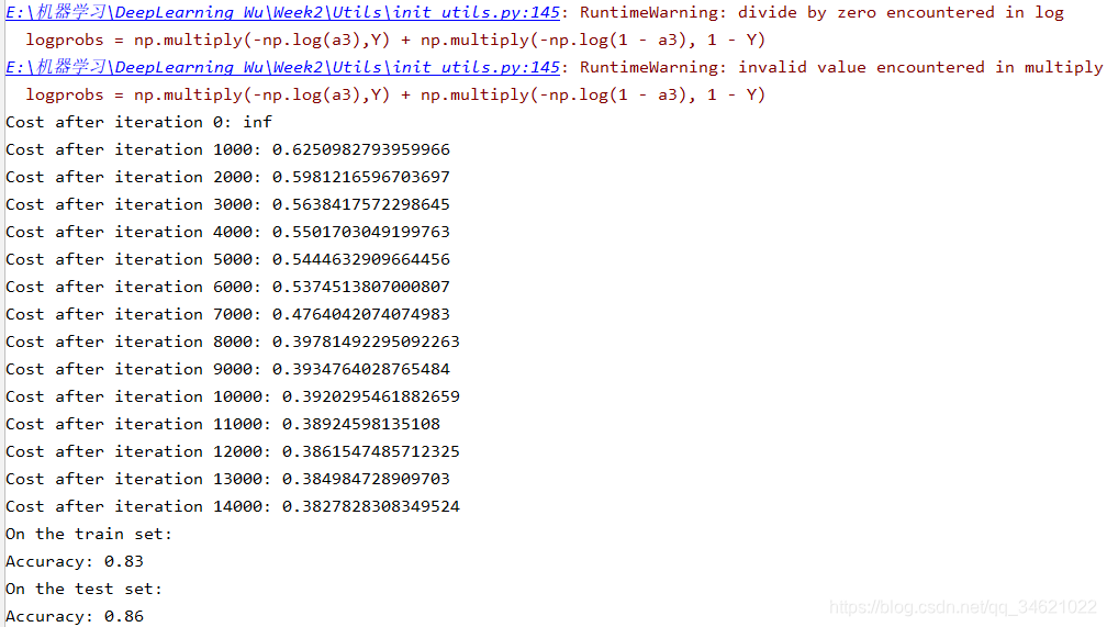
如果将“inf”视为迭代0之后的成本，这是因为数值舍入;更复杂的数字实现可以解决这个问题，我们不需要为报出的警告担心。
接下来我们打印一下预测结果，并用视图的方式查看分类效果：
代码：

    print(predictions_train)
    print(predictions_test)
    plt.title("Model with large random initialization")
    axes = plt.gca()
    axes.set_xlim([-1.5, 1.5])
    axes.set_ylim([-1.5, 1.5])
    plot_decision_boundary(lambda x: predict_dec(parameters, x.T), train_X, train_Y)

结果：


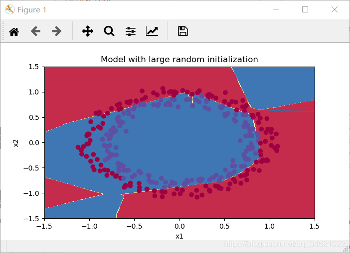
总结：
较大的权重会使得激活值非常接近于1或0（参考tanh函数曲线进行思考），当出现错误时会造成较大的损失，比如$log(a^{[3]})=log(0)$。
糟糕的初始化会导致渐变消失或爆炸，这也会减慢优化算法的速度。
如果你训练这个网络的时间更长，你会看到更好的结果，但初始化过大的随机数会减慢优化。
将权值初始化为非常大的随机值并不能很好地工作，用小的随机值初始化会更好。重要的问题是:这些随机值应该有多小?让我们在下一部分中找出答案吧!

1.23 He参数初始化

He初始化这个名字来源于2015年发表的论文的第一个作者名。Xavier初始化和He初始化大致相同，只不过Xavier初始化对权重$W^{[l]}$使用了比例因子$sqrt(1./layers_dims[l-1]) $,而He使用的是 sqrt(2./layers_dims[l-1])。
代码：

def initialize_parameters_he(layer_dims):
    np.random.seed(3)
    parameters = {}
    L = len(layer_dims)

    for l in range(1, L):
        parameters['W' + str(l)] = np.random.randn(layer_dims[l], layer_dims[l - 1]) * np.sqrt(2 / layer_dims[l - 1])
        parameters['b' + str(l)] = np.zeros((layer_dims[l], 1))

    return parameters

调用：

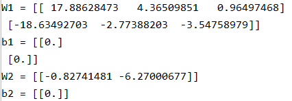
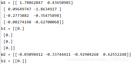
    parameters = initialize_parameters_he([2, 4, 1])
    print("W1 = " + str(parameters["W1"]))
    print("b1 = " + str(parameters["b1"]))
    print("W2 = " + str(parameters["W2"]))
    print("b2 = " + str(parameters["b2"]))

运行结果：

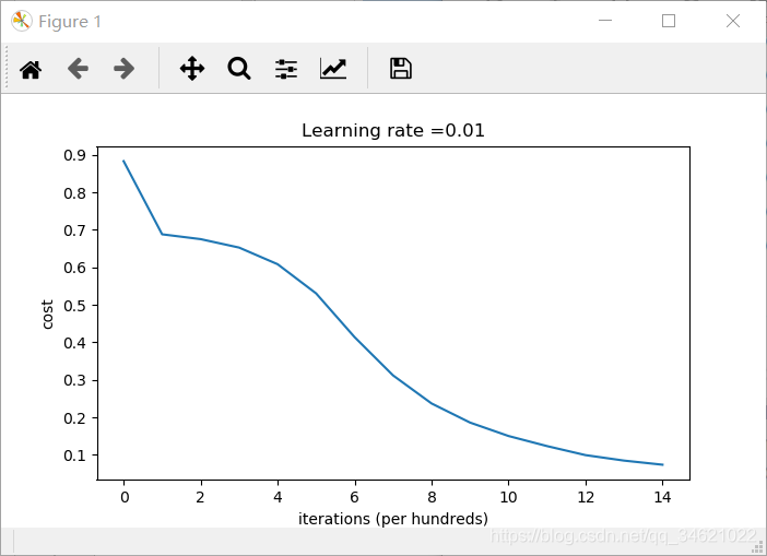
运用到三层神经网络模型中：
代码：

    parameters = model(train_X, train_Y, initialization="he")
    print("On the train set:")
    predictions_train = predict(train_X, train_Y, parameters)
    print("On the test set:")
    predictions_test = predict(test_X, test_Y, parameters)

运行结果：


查看分类效果：

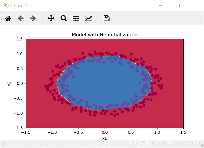
1.3 总结与归纳

我们在这一小节中使用了三种方法进行参数初始化：
1.零初始化：训练精度50% 很难打破对称性
2.随机初始化（较大值）：训练精度83% 可能会造成权重很大，造成梯度消失
3.He初始化：训练精度99% 推荐方法

2. 正则化

正则化的目的是为了解决过拟合问题。解决过拟合问题的方法经常使用有扩展数据集，但是有的时候数据集的获取成本过高，比如计算机视觉中获取某些图像数据集，因此在这里我们将学习一种新的解决过拟合的方法。
题目：
假设你是法国足球对雇佣的一名人工智能专家，他们希望你推荐法国队守门员应该踢球的位置，这样法国队的球员就可以用他们的头击球。用做题的角度看，就是有两类点，希望你尽可能的将其分开，在一类里面发球才能更大可能的被自己的同类接到。

2.1 加载数据集

每个点对应的是足球场上的一个位置，在法国守门员从足球场地左侧射门后，足球运动员用头部击球。

• 如果圆点是蓝色的，则表示法国队队员成功地用头击球
• 如果圆点是红色的，则表示对方球员用头部击球
  你的目标:使用一个深度学习模型来找到守门员应该踢球的位置。
  首先我们将数据可视化（调用的代码会放在文章最后）：
  代码：

    train_X, train_Y, test_X, test_Y = load_2D_dataset()

运行结果：

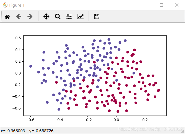
数据集的分析:这个数据集有点小噪音，但它看起来像一条对角线，将左上角(蓝色)和右下角(红色)分隔开，效果很好。
我们首先尝试一个非正则化模型。然后将学习如何规范它，并决定将选择哪种模式来解决法国足球公司的问题。

2.2正则化

2.21 非正则化模型

我们要使用的神经网络模型已经被吴恩达老师实现好了，需要注意的是，模型中有一个lambd参数（注意不要写成lambda，因为lambda是python中的一个关键字），当lambd不为零时，表示使用正则化，为零时不使用正则化。
代码：

def model(X, Y, learning_rate = 0.3, num_iterations = 30000, print_cost = True, lambd = 0, keep_prob = 1):
    """
    三层神经网络模型: LINEAR->RELU->LINEAR->RELU->LINEAR->SIGMOID.
    :param X: 输入的数据
    :param Y: 输出的数据
    :param learning_rate: 学习率
    :param num_iterations:迭代次数
    :param print_cost:是否打印代价
    :param lambd:正则化参数
    :param keep_prob:神经元在drop-out过程中保持活跃的概率，标量。
    :return:
    """
    grads = {}
    costs = []
    m = X.shape[1]
    layers_dims = [X.shape[0], 20, 3, 1]
    #1.初始化参数
    parameters = initialize_parameters(layers_dims)

    for i in range(0, num_iterations):
        #2.前向传播
        if keep_prob == 1:
            a3, cache = forward_propagation(X, parameters)
        # elif keep_prob < 1:
        #     a3, cache = forward_propagation_with_dropout(X, parameters, keep_prob)

        #3.计算代价
        if lambd == 0:
            cost = compute_cost(a3, Y)
        # else:
        #     cost = compute_cost_with_regularization(a3, Y, parameters, lambd)

        #4.反向传播
        #防止同时使用dropout和正则化
        assert (lambd == 0 or keep_prob == 1)
        if lambd == 0 and keep_prob == 1:
            grads = backward_propagation(X, Y, cache)
        # elif lambd != 0:
        #     grads = backward_propagation_with_regularization(X, Y, cache, lambd)
        # elif keep_prob < 1:
        #     grads = backward_propagation_with_dropout(X, Y, cache, keep_prob)

        #5.更新参数
        parameters = update_parameters(parameters, grads, learning_rate)

        if print_cost and i % 10000 == 0:
            print("Cost after iteration {}: {}".format(i, cost))
        if print_cost and i % 1000 == 0:
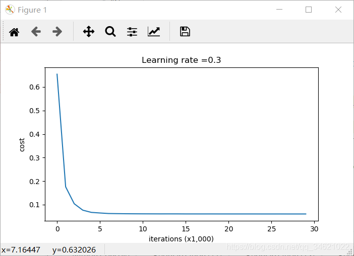
            costs.append(cost)

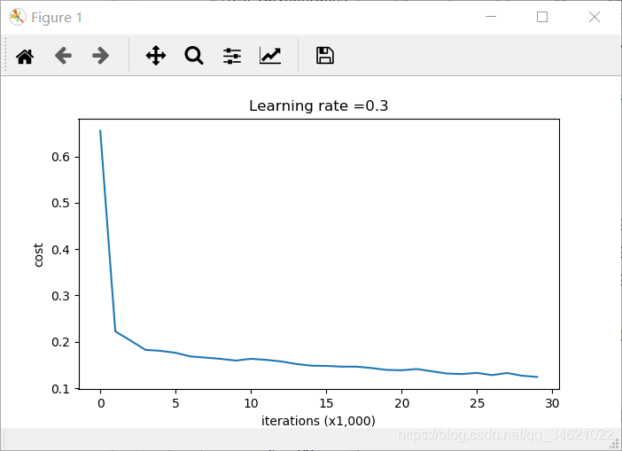
    plt.plot(costs)
    plt.ylabel('cost')
    plt.xlabel('iterations (x1,000)')
    plt.title("Learning rate =" + str(learning_rate))
    plt.show()

    return parameters

调用：

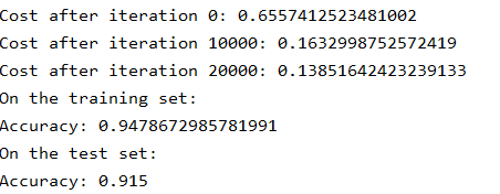
    parameters = model(train_X, train_Y)
    print("On the training set:")
    predictions_train = predict(train_X, train_Y, parameters)
    print("On the test set:")
    predictions_test = predict(test_X, test_Y, parameters)

运行结果：


这是基线模型(我们将观察正则化对该模型的影响)。运行以下代码来绘制模型的决策边界。
代码：

    axes = plt.gca()
    axes.set_xlim([-0.75, 0.40])
    axes.set_ylim([-0.75, 0.65])
    plot_decision_boundary(lambda x: predict_dec(parameters, x.T), train_X, train_Y)

运行结果：

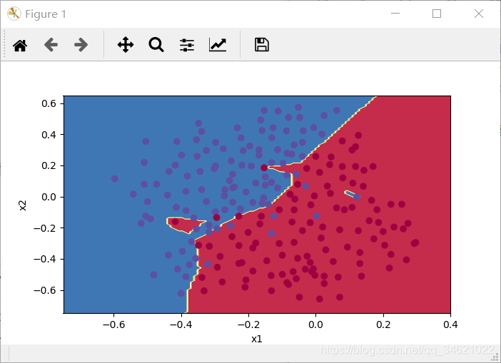
训练集精度明显高于测试集精度，非正则化模型对训练集的过度拟合，这是对噪声点的拟合。现在让我们实现减少过度拟合的两种技术。

2.22 L2-正则化

避免过度拟合的标准方法称为L2正则化。
它的主要特点在对代价函数的修改上，加上在正则化项以后相当于对权重矩阵有了一个惩罚。
$$J=-\frac{1}{m}\sum _{i=1}^m(y^{(i)}\log \left(a^{[L](i)}\right)+(1-y^{(i)})\log \left(1-a^{[L](i)}\right))$$ To: $$J_{regularized}=\underset{\text{cross-entropy cost}}{\underbrace{-\frac{1}{m}\sum _{i=1}^m(y^{(i)}\log \left(a^{[L](i)}\right)+(1-y^{(i)})\log \left(1-a^{[L](i)}\right))}}+\underset{\text{L2 regularization cost}}{\underbrace{\frac{1}{m}\frac{\lambda }{2}\sum _l\sum _k\sum _j{W}_{k,j}^{[l]2}}}$$
接下来实现compute_cost_with_regularization()，计算$\sum _k\sum _j{W}_{k,j}^{[l]2}$ ，使用np.sum(np.square(Wl))
代码：

def compute_cost_with_regularization(A3, Y, parameters, lambd):
    """
    :param A3: 激活值
    :param Y: 标签
    :param parameters:
    :return: 记录每轮的代价
    """
    m = Y.shape[1]
    W1 = parameters["W1"]
    W2 = parameters["W2"]
    W3 = parameters["W3"]

    cross_entropy_cost = compute_cost(A3, Y)

    L2_regularization_cost = lambd * (np.sum(np.square(W1)) + np.sum(np.square(W2)) + np.sum(np.square(W3))) / (2 * m)

    cost = cross_entropy_cost + L2_regularization_cost

    return cost

调用代码：

    A3, Y_assess, parameters = compute_cost_with_regularization_test_case()
    
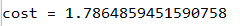
    print("cost = " + str(compute_cost_with_regularization(A3, Y_assess, parameters, lambd=0.1)))  

运行结果：

实现反向传播中需要的更改，以实现正则化。这些变化只与dW1、dW2和dW3有关。对于每一个，您必须添加正则化项的梯度($\frac{d}{dW}(\frac{1}{2}\frac{\lambda }{m}{W}^2)=\frac{\lambda }{m}W$)。

代码：

def backward_propagation_with_regularization(X, Y, cache, lambd):
    m = X.shape[1]
    (Z1, A1, W1, b1, Z2, A2, W2, b2, Z3, A3, W3, b3) = cache

    dZ3 = A3 - Y
    dW3 = 1. / m * np.dot(dZ3, A2.T) + (lambd * W3) / m
    db3 = 1. / m * np.sum(dZ3, axis=1, keepdims=True)
    dA2 = np.dot(W3.T, dZ3)

    dZ2 = np.multiply(dA2, np.int64(A2 > 0))
    dW2 = 1. / m * np.dot(dZ2, A1.T) + (lambd * W2) / m
    db2 = 1. / m * np.sum(dZ2, axis=1, keepdims=True)

    dA1 = np.dot(W2.T, dZ2)
    dZ1 = np.multiply(dA1, np.int64(A1 > 0))
    dW1 = 1. / m * np.dot(dZ1, X.T) + (lambd * W1) / m
    db1 = 1. / m * np.sum(dZ1, axis=1, keepdims=True)

    gradients = {"dZ3": dZ3, "dW3": dW3, "db3": db3, "dA2": dA2,
                 "dZ2": dZ2, "dW2": dW2, "db2": db2, "dA1": dA1,
                 "dZ1": dZ1, "dW1": dW1, "db1": db1}

    return gradients

调用：

    X_assess, Y_assess, cache = backward_propagation_with_regularization_test_case()

    grads = backward_propagation_with_regularization(X_assess, Y_assess, cache, lambd=0.7)
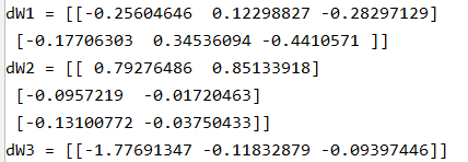
    print("dW1 = " + str(grads["dW1"]))
    print("dW2 = " + str(grads["dW2"]))
    print("dW3 = " + str(grads["dW3"]))

运行结果：

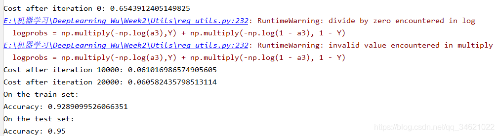
使用L2-正则化方式运行模型，其中lambd = 0.7：

parameters = model(train_X, train_Y, lambd=0.7)
print("On the train set:")
predictions_train = predict(train_X, train_Y, parameters)
print("On the test set:")
predictions_test = predict(test_X, test_Y, parameters)

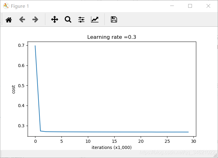
运行结果：

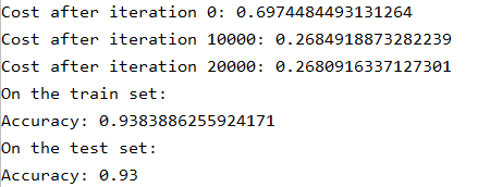
可以看到测试集的准确率已经达到了93%。

画一下分类边界。

    plt.title("Model with L2-regularization")
    axes = plt.gca()
    axes.set_xlim([-0.75, 0.40])
    axes.set_ylim([-0.75, 0.65])
    plot_decision_boundary(lambda x: predict_dec(parameters, x.T), train_X, train_Y)

运行结果：

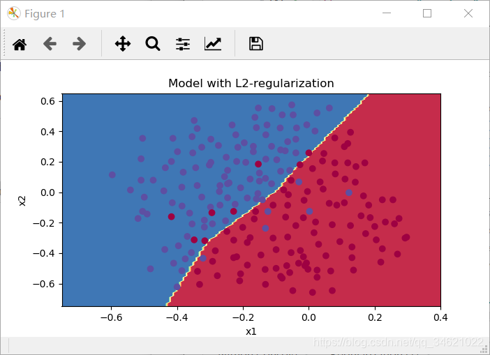
注意：

• $\lambda$的值是一个超参数，可以使用训练集对其进行调优。
• L2正则化使决策边界更平滑。如果$\lambda$太大，也有可能“过度平滑”，导致模型具有较高的偏差。
  L2正则化依赖于这样一个假设，即具有小权值的模型比具有大权值的模型更简单。因此，通过惩罚成本函数中权值的平方值，您可以将所有权值转换为更小的值。这导致了一个更平滑的模型，其中输出随着输入的变化而变化得更慢。

2.23 Dropout

dropout是一种广泛使用的正则化技术，专门针对深度学习。它会在每次迭代中随机关闭一些神经元。
你关闭一些神经元时，实际上是在修改你的模型。drop-out背后的思想是，在每次迭代中，训练一个不同的模型，该模型只使用你的神经元的一个子集。随着神经元的缺失，你的神经元对另一个特定神经元的激活变得不那么敏感，因为那个特定神经元可能随时会被关闭。

使用Dropout的正向传播
练习：使用dropout实现正向传播。使用一个3层的神经网络，并将dropout添加到第一和第二隐藏层。我们将不应用dropout到输入层或输出层。

关闭第一层和第三层的一些节点，我们通常需要分以下四个步骤完成：
1.使用np.random.randn()生成一个和$a^{[l]}$具有相同维数的$d^{[l]}$,使用向量来表示就是$D^{[1]}=[d^{[l](1)}{d}^{[l](2)}...d^{[l](m)}]$和$A^{[l]}$的维数相同。
2.如果$D^{[l]}$低于keep_prob的值就设为0，高于设为1.
3.更新$A^{[l]}$的值，将其值更新为$A^l\ast D^l$。
4.$A^{[l]}$的值需要除以keep_prob，这样计算成本时仍有相同的期望值，这也成为Inverted-dropout。

代码：

def forward_propagation_with_dropout(X, parameters, keep_prob=0.5):
    """
    前向传播模型： LINEAR -> RELU + DROPOUT -> LINEAR -> RELU + DROPOUT -> LINEAR -> SIGMOID.
    :param X:训练数据集
    :param parameters:"W1", "b1", "W2", "b2", "W3", "b3":
                    W1 -- 权重矩阵维数 (20, 2)
                    b1 -- 偏置矩阵维数 (20, 1)
                    W2 -- 权重矩阵维数 (3, 20)
                    b2 -- 偏置矩阵维数 (3, 1)
                    W3 -- 权重矩阵维数 (1, 3)
                    b3 -- 偏置矩阵维数 (1, 1)
    :param keep_prob:删除节点的概率
    :return:
        A3：最后一层的激活值，维数为（1， 1）
        cache：存储了一些用于计算反向传播的数值元组。
    """
    np.random.seed(1)
    W1 = parameters["W1"]
    b1 = parameters["b1"]
    W2 = parameters["W2"]
    b2 = parameters["b2"]
    W3 = parameters["W3"]
    b3 = parameters["b3"]

    Z1 = np.dot(W1, X) + b1
    A1 = relu(Z1)
    #1.初始化随机矩阵
    D1 = np.random.rand(A1.shape[0], A1.shape[1])
    #2.将矩阵值根据keep_prob的值比较，转换为0，1，实质上就是做一个判断，返回true和false
    D1 = D1 < keep_prob
    #3.更新A激活矩阵的值
    A1 = A1 * D1
    #4. 缩放舍弃0的值，保证期望值相同
    A1 = A1 / keep_prob

    #按照上述步骤计算第二层
    Z2 = np.dot(W2, A1) + b2
    A2 = relu(Z2)
    D2 = np.random.rand(A2.shape[0], A2.shape[1])
    D2 = D2 < keep_prob
    A2 = A2 * D2
    A2 = A2 / keep_prob

    #输入层和输出层不做处理
    Z3 = np.dot(W3, A2) + b3
    A3 = sigmoid(Z3)

    cache = (Z1, D1, A1, W1, b1, Z2, D2, A2, W2, b2, Z3, A3, W3, b3)

    return A3, cache

调用：

    X_assess, parameters = forward_propagation_with_dropout_test_case()

    A3, cache = forward_propagation_with_dropout(X_assess, parameters, keep_prob=0.7)
    print("A3 = " + str(A3))

运行结果：

使用dropout的反向传播
练习:使用dropout实现反向传播。如前所述，训练的是一个3层网络。使用缓存中存储的掩码$D^{[1]}$和$D^{[2]}$，将dropout添加到第一个和第二个隐藏层。

使用dropout的反向传播一般分以下两个步骤完成:
1.之前我们在正向传播中使用$D^{[l]}$关闭了一些神经单元。在反向传播中，我们也需要关闭相同的神经元，方法是将相同的掩码$D^{[1]}$重新应用于dA1。
2.在正向传播过程中，A1除以keep_prob。因此，在反向传播中，必须将dA1除以keep_prob(微积分上的解释是，如果$A^{[1]}$被keep_prob缩放，那么它的导数$d{A}^{[1]}$也被相同的keep_prob缩放)。
代码：

def backward_propagation_with_dropout(X, Y, cache, keep_prob):
    """
    :param X: 输入的数据集
    :param Y: 输入数据集对应的分类标签
    :param cache: 前向传播中返回的参数
    :param keep_prob: 删除率
    :return: gradients
    """
    m = X.shape[1]
    (Z1, D1, A1, W1, b1, Z2, D2, A2, W2, b2, Z3, A3, W3, b3) = cache
    dZ3 = A3 - Y
    dW3 = 1. / m * np.dot(dZ3, A2.T)
    db3 = 1. / m * np.sum(dZ3, axis=1, keepdims=True)
    dA2 = np.dot(W3.T, dZ3)
    dA2 = dA2 / keep_prob

    dZ2 = np.multiply(dA2, np.int64(A2 > 0))
    dW2 = 1. / m * np.dot(dZ2, A1.T)
    db2 = 1. / m * np.sum(dZ2, axis=1, keepdims=True)
    dA1 = np.dot(W2.T, dZ2)
    dA1 = dA1 * D1
    dA1 = dA1 / keep_prob

    dZ1 = np.multiply(dA1, np.int64(A1 > 0))
    dW1 = 1. / m * np.dot(dZ1, X.T)
    db1 = 1. / m * np.sum(dZ1, axis=1, keepdims=True)

    gradients = {"dZ3": dZ3, "dW3": dW3, "db3": db3, "dA2": dA2,
                 "dZ2": dZ2, "dW2": dW2, "db2": db2, "dA1": dA1,
                 "dZ1": dZ1, "dW1": dW1, "db1": db1}

    return gradients

调用：

    X_assess, Y_assess, cache = backward_propagation_with_dropout_test_case()

    gradients = backward_propagation_with_dropout(X_assess, Y_assess, cache, keep_prob=0.8)

    print("dA1 = " + str(gradients["dA1"]))
    print("dA2 = " + str(gradients["dA2"]))

运行结果：

现在让我们用dropout (keep_prob = 0.86)运行模型。这意味着在每次迭代中，关闭第1层和第2层神经元的概率是24%。函数模型()现在将调用:
代码：

    parameters = model(train_X, train_Y, keep_prob=0.86, learning_rate=0.3)

    print("On the train set:")
    predictions_train = predict(train_X, train_Y, parameters)
    print("On the test set:")
    predictions_test = predict(test_X, test_Y, parameters)

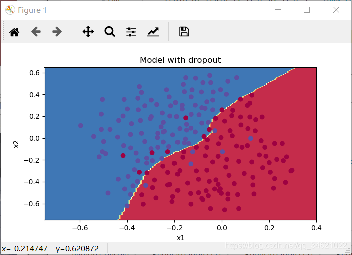
运行结果：


查看分类边界：

    plt.title("Model with dropout")
    axes = plt.gca()
    axes.set_xlim([-0.75, 0.40])
    axes.set_ylim([-0.75, 0.65])
    plot_decision_boundary(lambda x: predict_dec(parameters, x.T), train_X, train_Y)

注意：
使用dropout的一个常见错误是在训练和测试时中都使用它，其实我们值需要在训练时使用dropout就可以。
在正向传播和反向传播中都需要使用dropout。
在训练期间，通过keep_prob将每个dropout层划分为相同的激活期望值。例如，如果keep_prob为0.5，那么我们将平均关闭一半的节点，因此输出将按0.5进行伸缩，因为只有剩下的一半对解决方案有贡献。除以0.5等于乘以2。因此，输出现在具有相同的期望值。

2.3 总结与归纳

模型	训练精度	测试精度
没有使用正则化的三层神经网络模型	95%	91.5%
使用L2正则化的三层神经网络模型	94%	93%
使用dropout的三层神经网络模型	93%	95%

注意，正则化会影响训练集的性能，因为它限制了网络对训练集的过度适应能力。但是它最终提供了更好的测试准确性。

3. 梯度检验

题目背景：
你属于一个致力于在全球范围内提供移动支付的公司,你的工作是建立一个深度学习模型来检测欺诈,每当有人支付就判断付款是否虚假的，比如用户的帐户已经被黑客控制。
但是反向传播的实现非常具有挑战性，有时还会有bug。因为这是一个任务关键型应用程序，所以公司的CEO希望确保反向传播的实现是正确的。你的CEO说，“你需要给我证明你的反向传播实际上是能正确工作的!”为了保证这一点，您将使用“梯度检查”。

3.1 怎样进行梯度检验

反向传播计算梯度$\frac{\partial J}{\partial \theta }$，其中$\theta$表示模型的参数。$J$是使用正向传播和损失函数计算的。
因为前向传播相对容易实现，所以您对自己做对了很有信心，所以您几乎100%肯定自己正确地计算了成本$J$。因此，您可以使用计算$J$的代码来验证计算$\frac{\partial J}{\partial \theta }$的代码。
让我们回顾一下导数(或梯度)的定义:$$\frac{\partial J}{\partial \theta }=\underset{\epsilon \to 0}{\lim }\frac{J(\theta +\epsilon )-J(\theta -\epsilon )}{2\epsilon }$$

3.2 梯度检验实现

3.21 一维模型梯度检验

考虑一个一维线性函数$J(\theta )=\theta x$。该模型只包含一个实值参数$\theta$，并接受$x$作为输入。
您将实现计算$J(.)$及其导数$\frac{\partial J}{\partial \theta }$的代码。然后使用梯度检查来确保对$J$的导数计算是正确的。

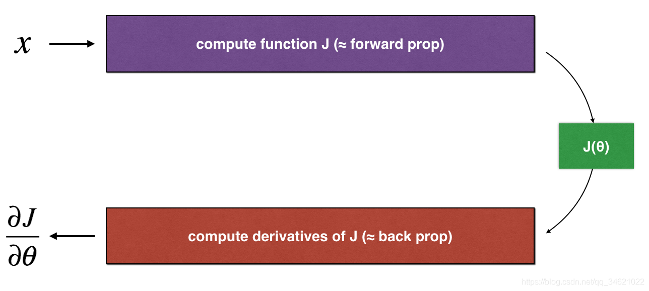
上面的图表显示了计算步骤:首先从$x$开始，然后计算函数$J(x)$(“正向传播”)。再计算导数$\frac{\partial J}{\partial \theta }$(“反向传播”)。

以这个线性模型为例实现梯度检验：
模仿正向传播代码：

def forward_propagation(x, theta):
    J = np.dot(theta, x)
    return J

if __name__ == "__main__":
    x, theta = 2, 4
    J = forward_propagation(x, theta)
    print("J = " + str(J))

运行结果：

模仿反向传播：计算$J(\theta )=\theta x$对$\theta$的导数,我们应该得到$d\theta =\frac{\partial J}{\partial \theta }=x$。
代码：

def backward_propagation(x, theta):
    dtheta = x

    return dtheta
    
if __name__ == "__main__":
    x, theta = 2, 4
    dtheta = backward_propagation(x, theta)
    print("dtheta = " + str(dtheta))

运行结果：

为了显示backward_propagation()函数正确地计算了梯度值$\frac{\partial J}{\partial \theta }$，让我们实现梯度检查。

步骤
1.首先使用上面的公式和值$\epsilon$,计算“gradapprox”。以下是需要采取的步骤:
${\theta }^{+}=\theta +\epsilon$
${\theta }^{-}=\theta -\epsilon$
$J^{+}=J({\theta }^{+})$
$J^{-}=J({\theta }^{-})$
$gradapprox$ = $\frac{J^{+}-J^{-}}{2\epsilon }$
2.使用反向传播计算梯度，并将结果存储在变量“grad”中。
3.使用以下公式计算“gradapprox”和“grad”之间的相对差异
$$difference=\frac{\mid \mid grad-gradapprox\mid {\mid }_2}{\mid \mid grad\mid {\mid }_2+\mid \mid gradapprox\mid {\mid }_2}$$

代码：

def gradient_check(x, theta, epsilon=1e-7):
    thetaplus = theta + epsilon
    thetaminus = theta - epsilon
    J_plus = forward_propagation(x, thetaplus)
    J_minus = forward_propagation(x, thetaminus)
    gradapprox = (J_plus - J_minus) / (2 * epsilon)

    grad = backward_propagation(x, theta)

    numerator = np.linalg.norm(grad - gradapprox)
    denominator = np.linalg.norm(grad) + np.linalg.norm(gradapprox)
    difference = numerator / denominator

    if difference < 1e-7:
        print("梯度正确")
    else:
        print("梯度错误!")

    return difference

调用:

    x, theta = 2, 4
    difference = gradient_check(x, theta)
    print("difference = " + str(difference))

运行结果:

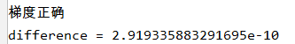
这个差值小于阈值$10^{(-7)}$。因此，我们可以确信自己已经正确地计算了backward_propagation()中的梯度。

3.22 N维模型梯度检验

下面的图片很好的阐述了N-维模型梯度检验的过程。

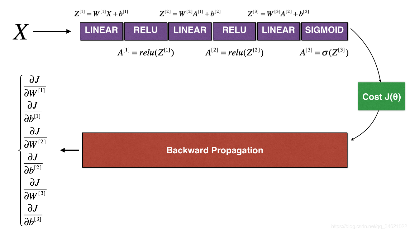
正向传播
代码：

def backward_propagation_n(X, Y, cache):
    m = X.shape[1]
    (Z1, A1, W1, b1, Z2, A2, W2, b2, Z3, A3, W3, b3) = cache

    dZ3 = A3 - Y
    dW3 = 1. / m * np.dot(dZ3, A2.T)
    db3 = 1. / m * np.sum(dZ3, axis = 1, keepdims=True)

    dA2 = np.dot(W3.T, dZ3)
    dZ2 = np.multiply(dA2, np.int64(A2 > 0))
    dW2 = 1. / m * np.dot(dZ2, A1.T) * 2
    db2 = 1. / m * np.sum(dZ2, axis=1, keepdims = True)

    dA1 = np.dot(W2.T, dZ2)
    dZ1 = np.multiply(dA1, np.int64(A1 > 0))
    dW1 = 1. / m * np.dot(dZ1, X.T)
    db1 = 4. / m * np.sum(dZ1, axis=1, keepdims=True)  # Should not multiply by 4

    gradients = {"dZ3": dZ3, "dW3": dW3, "db3": db3,
                 "dA2": dA2, "dZ2": dZ2, "dW2": dW2, "db2": db2,
                 "dA1": dA1, "dZ1": dZ1, "dW1": dW1, "db1": db1}

    return gradients

接下来我们使用下面的公式来进行梯度验证：
$$\frac{\partial J}{\partial \theta }=\underset{\epsilon \to 0}{\lim }\frac{J(\theta +\epsilon )-J(\theta -\epsilon )}{2\epsilon }$$
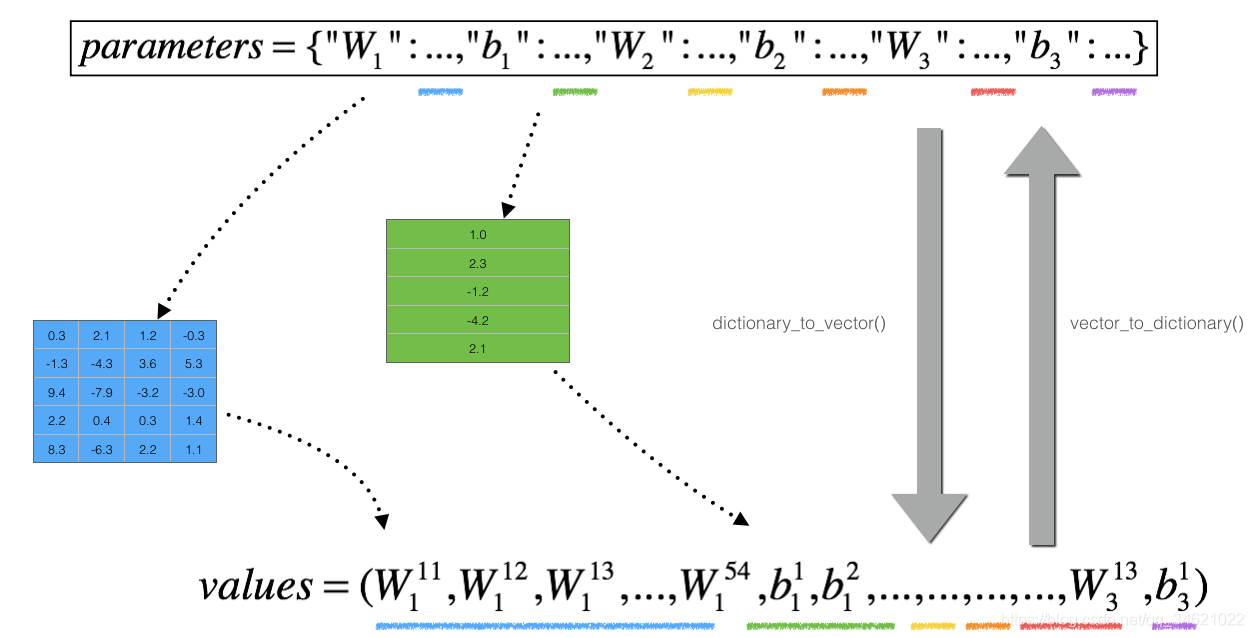
但是，$\theta$不再是一个标量。这是一个叫做“parameters”的字典类型。吴老师为我们实现了一个函数“dictionary_to_vector()”。它将“parameters”字典转换为一个称为“values”的向量，通过将所有参数(W1、b1、W2、b2、W3、b3)重新整形为向量并将它们连接起来。
具体过程如下图所示：

N层模型上进行梯度检验：
对于num_parameters中的每个i有：

• 计算$J_{p}lus[i]$:
• 1.设置${\theta }^{+}$为np.copy(parameters_values)
• 2.设置${\theta }_i^{+}$为${\theta }_i^{+}+\epsilon$
• 3.使用foreard_propagation_n(x, y, vector_to_dictionary(${\theta }^{+}$))来计算$J_i^{+}$
• 计算J_minus[i]:使用相同的方法计算${\theta }^{-}$
• 计算$gradapprox[i]=\frac{J_i^{+}-J_i^{-}}{2\epsilon }$
• 计算误差：
• 计算梯度
  $$difference=\frac{\mid \mid grad-gradapprox\mid {\mid }_2}{\mid \mid grad\mid {\mid }_2+\mid \mid gradapprox\mid {\mid }_2}$$

代码：

def gradient_check_n(parameters, gradients, X, Y, epsilon=1e-7):
    parameters_values, _ = dictionary_to_vector(parameters)
    grad = gradients_to_vector(gradients)
    num_parameters = parameters_values.shape[0]
    J_plus = np.zeros((num_parameters, 1))
    J_minus = np.zeros((num_parameters, 1))
    gradapprox = np.zeros((num_parameters, 1))

    for i in range(num_parameters):
        thetaplus = np.copy(parameters_values)
        thetaplus[i][0] = thetaplus[i][0] + epsilon
        J_plus[i], _ = forward_propagation_n(X, Y, vector_to_dictionary(thetaplus))

        thetaminus = np.copy(parameters_values)
        thetaminus[i][0] = thetaminus[i][0] - epsilon
        J_minus[i], _ = forward_propagation_n(X, Y, vector_to_dictionary(thetaminus))

        gradapprox[i] = (J_plus[i] - J_minus[i]) / (2 * epsilon)

    numerator = np.linalg.norm(grad - gradapprox)
    denominator = np.linalg.norm(grad) + np.linalg.norm(gradapprox)
    difference = numerator / denominator

    if difference > 1e-7:
        print("你的反向传播有错误，误差 = " + str(difference))
    else:
        print("你的反向传播工作的很好，误差 = " + str(difference))

    return difference

调用：

    X, Y, parameters = gradient_check_n_test_case()

    cost, cache = forward_propagation_n(X, Y, parameters)
    gradients = backward_propagation_n(X, Y, cache)
    difference = gradient_check_n(parameters, gradients, X, Y)

运行结果：

注意：

• 渐变检查很慢!使用$\frac{\partial J}{\partial \theta }\approx \frac{J(\theta +\epsilon )-J(\theta -\epsilon )}{2\epsilon }$来计算近似梯度值花费的代价很大。因此，我们不会在训练期间的每次迭代中都运行梯度检查。只要检查几次梯度是否正确就可以。
• 梯度检查不与dropout在一起使用。你通常会运行没有dropout的梯度检查算法，以确保你的反向传播是正确的，正确后再添加dropout。

使用的库函数：

1.init_utils.py

import numpy as np
import matplotlib.pyplot as plt
import h5py
import sklearn
import sklearn.datasets

def sigmoid(x):
    """
    Compute the sigmoid of x

    Arguments:
    x -- A scalar or numpy array of any size.

    Return:
    s -- sigmoid(x)
    """
    s = 1/(1+np.exp(-x))
    return s

def relu(x):
    """
    Compute the relu of x

    Arguments:
    x -- A scalar or numpy array of any size.

    Return:
    s -- relu(x)
    """
    s = np.maximum(0,x)
    
    return s

def forward_propagation(X, parameters):
    """
    Implements the forward propagation (and computes the loss) presented in Figure 2.
    
    Arguments:
    X -- input dataset, of shape (input size, number of examples)
    Y -- true "label" vector (containing 0 if cat, 1 if non-cat)
    parameters -- python dictionary containing your parameters "W1", "b1", "W2", "b2", "W3", "b3":
                    W1 -- weight matrix of shape ()
                    b1 -- bias vector of shape ()
                    W2 -- weight matrix of shape ()
                    b2 -- bias vector of shape ()
                    W3 -- weight matrix of shape ()
                    b3 -- bias vector of shape ()
    
    Returns:
    loss -- the loss function (vanilla logistic loss)
    """
        
    # retrieve parameters
    W1 = parameters["W1"]
    b1 = parameters["b1"]
    W2 = parameters["W2"]
    b2 = parameters["b2"]
    W3 = parameters["W3"]
    b3 = parameters["b3"]
    
    # LINEAR -> RELU -> LINEAR -> RELU -> LINEAR -> SIGMOID
    z1 = np.dot(W1, X) + b1
    a1 = relu(z1)
    z2 = np.dot(W2, a1) + b2
    a2 = relu(z2)
    z3 = np.dot(W3, a2) + b3
    a3 = sigmoid(z3)
    
    cache = (z1, a1, W1, b1, z2, a2, W2, b2, z3, a3, W3, b3)
    
    return a3, cache

def backward_propagation(X, Y, cache):
    """
    Implement the backward propagation presented in figure 2.
    
    Arguments:
    X -- input dataset, of shape (input size, number of examples)
    Y -- true "label" vector (containing 0 if cat, 1 if non-cat)
    cache -- cache output from forward_propagation()
    
    Returns:
    gradients -- A dictionary with the gradients with respect to each parameter, activation and pre-activation variables
    """
    m = X.shape[1]
    (z1, a1, W1, b1, z2, a2, W2, b2, z3, a3, W3, b3) = cache
    
    dz3 = 1./m * (a3 - Y)
    dW3 = np.dot(dz3, a2.T)
    db3 = np.sum(dz3, axis=1, keepdims = True)
    
    da2 = np.dot(W3.T, dz3)
    dz2 = np.multiply(da2, np.int64(a2 > 0))
    dW2 = np.dot(dz2, a1.T)
    db2 = np.sum(dz2, axis=1, keepdims = True)
    
    da1 = np.dot(W2.T, dz2)
    dz1 = np.multiply(da1, np.int64(a1 > 0))
    dW1 = np.dot(dz1, X.T)
    db1 = np.sum(dz1, axis=1, keepdims = True)
    
    gradients = {"dz3": dz3, "dW3": dW3, "db3": db3,
                 "da2": da2, "dz2": dz2, "dW2": dW2, "db2": db2,
                 "da1": da1, "dz1": dz1, "dW1": dW1, "db1": db1}
    
    return gradients

def update_parameters(parameters, grads, learning_rate):
    """
    Update parameters using gradient descent
    
    Arguments:
    parameters -- python dictionary containing your parameters 
    grads -- python dictionary containing your gradients, output of n_model_backward
    
    Returns:
    parameters -- python dictionary containing your updated parameters 
                  parameters['W' + str(i)] = ... 
                  parameters['b' + str(i)] = ...
    """
    
    L = len(parameters) // 2 # number of layers in the neural networks

    # Update rule for each parameter
    for k in range(L):
        parameters["W" + str(k+1)] = parameters["W" + str(k+1)] - learning_rate * grads["dW" + str(k+1)]
        parameters["b" + str(k+1)] = parameters["b" + str(k+1)] - learning_rate * grads["db" + str(k+1)]
        
    return parameters

def compute_loss(a3, Y):
    
    """
    Implement the loss function
    
    Arguments:
    a3 -- post-activation, output of forward propagation
    Y -- "true" labels vector, same shape as a3
    
    Returns:
    loss - value of the loss function
    """
    
    m = Y.shape[1]
    logprobs = np.multiply(-np.log(a3),Y) + np.multiply(-np.log(1 - a3), 1 - Y)
    loss = 1./m * np.nansum(logprobs)
    
    return loss

def load_cat_dataset():
    train_dataset = h5py.File('../dataSets/train_catvnoncat.h5', "r")
    train_set_x_orig = np.array(train_dataset["train_set_x"][:]) # your train set features
    train_set_y_orig = np.array(train_dataset["train_set_y"][:]) # your train set labels

    test_dataset = h5py.File('../dataSets/test_catvnoncat.h5', "r")
    test_set_x_orig = np.array(test_dataset["test_set_x"][:]) # your test set features
    test_set_y_orig = np.array(test_dataset["test_set_y"][:]) # your test set labels

    classes = np.array(test_dataset["list_classes"][:]) # the list of classes
    
    train_set_y = train_set_y_orig.reshape((1, train_set_y_orig.shape[0]))
    test_set_y = test_set_y_orig.reshape((1, test_set_y_orig.shape[0]))
    
    train_set_x_orig = train_set_x_orig.reshape(train_set_x_orig.shape[0], -1).T
    test_set_x_orig = test_set_x_orig.reshape(test_set_x_orig.shape[0], -1).T
    
    train_set_x = train_set_x_orig/255
    test_set_x = test_set_x_orig/255

    return train_set_x, train_set_y, test_set_x, test_set_y, classes


def predict(X, y, parameters):
    """
    This function is used to predict the results of a  n-layer neural network.
    
    Arguments:
    X -- data set of examples you would like to label
    parameters -- parameters of the trained model
    
    Returns:
    p -- predictions for the given dataset X
    """
    
    m = X.shape[1]
    p = np.zeros((1, m), dtype = np.int)
    
    # Forward propagation
    a3, caches = forward_propagation(X, parameters)
    
    # convert probas to 0/1 predictions
    for i in range(0, a3.shape[1]):
        if a3[0,i] > 0.5:
            p[0,i] = 1
        else:
            p[0,i] = 0

    # print results
    print("Accuracy: "  + str(np.mean((p[0,:] == y[0,:]))))
    
    return p

def plot_decision_boundary(model, X, y):
    # Set min and max values and give it some padding
    x_min, x_max = X[0, :].min() - 1, X[0, :].max() + 1
    y_min, y_max = X[1, :].min() - 1, X[1, :].max() + 1
    h = 0.01
    # Generate a grid of points with distance h between them
    xx, yy = np.meshgrid(np.arange(x_min, x_max, h), np.arange(y_min, y_max, h))
    # Predict the function value for the whole grid
    Z = model(np.c_[xx.ravel(), yy.ravel()])
    Z = Z.reshape(xx.shape)
    # Plot the contour and training examples
    plt.contourf(xx, yy, Z, cmap=plt.cm.Spectral)
    plt.ylabel('x2')
    plt.xlabel('x1')
    plt.scatter(X[0, :], X[1, :], c=np.squeeze(y), cmap=plt.cm.Spectral)
    plt.show()
    
def predict_dec(parameters, X):
    """
    Used for plotting decision boundary.
    
    Arguments:
    parameters -- python dictionary containing your parameters 
    X -- input data of size (m, K)
    
    Returns
    predictions -- vector of predictions of our model (red: 0 / blue: 1)
    """
    
    # Predict using forward propagation and a classification threshold of 0.5
    a3, cache = forward_propagation(X, parameters)
    predictions = (a3 > 0.5)
    return predictions

def load_dataset():
    np.random.seed(1)
    train_X, train_Y = sklearn.datasets.make_circles(n_samples=300, noise=.05)
    print(train_X.shape)
    print(train_Y.shape)
    np.random.seed(2)
    #train_X.shape=(300,2) train_Y.shape=(300,)
    test_X, test_Y = sklearn.datasets.make_circles(n_samples=100, noise=.05)
    # Visualize the data
    # plt.scatter(train_X[:, 0], train_X[:, 1], c=train_Y, s=40, cmap=plt.cm.Spectral);
    train_X = train_X.T
    train_Y = train_Y.reshape((1, train_Y.shape[0]))
    test_X = test_X.T
    test_Y = test_Y.reshape((1, test_Y.shape[0]))
    return train_X, train_Y, test_X, test_Y

2. reg_utils.py

import numpy as np
import matplotlib.pyplot as plt
import h5py
import sklearn
import sklearn.datasets
import sklearn.linear_model
import scipy.io

def sigmoid(x):
    """
    Compute the sigmoid of x

    Arguments:
    x -- A scalar or numpy array of any size.

    Return:
    s -- sigmoid(x)
    """
    s = 1/(1+np.exp(-x))
    return s

def relu(x):
    """
    Compute the relu of x

    Arguments:
    x -- A scalar or numpy array of any size.

    Return:
    s -- relu(x)
    """
    s = np.maximum(0,x)
    
    return s

def load_planar_dataset(seed):
    
    np.random.seed(seed)
    
    m = 400 # number of examples
    N = int(m/2) # number of points per class
    D = 2 # dimensionality
    X = np.zeros((m,D)) # data matrix where each row is a single example
    Y = np.zeros((m,1), dtype='uint8') # labels vector (0 for red, 1 for blue)
    a = 4 # maximum ray of the flower

    for j in range(2):
        ix = range(N*j,N*(j+1))
        t = np.linspace(j*3.12,(j+1)*3.12,N) + np.random.randn(N)*0.2 # theta
        r = a*np.sin(4*t) + np.random.randn(N)*0.2 # radius
        X[ix] = np.c_[r*np.sin(t), r*np.cos(t)]
        Y[ix] = j
        
    X = X.T
    Y = Y.T

    return X, Y

def initialize_parameters(layer_dims):
    """
    Arguments:
    layer_dims -- python array (list) containing the dimensions of each layer in our network
    
    Returns:
    parameters -- python dictionary containing your parameters "W1", "b1", ..., "WL", "bL":
                    W1 -- weight matrix of shape (layer_dims[l], layer_dims[l-1])
                    b1 -- bias vector of shape (layer_dims[l], 1)
                    Wl -- weight matrix of shape (layer_dims[l-1], layer_dims[l])
                    bl -- bias vector of shape (1, layer_dims[l])
                    
    Tips:
    - For example: the layer_dims for the "Planar Data classification model" would have been [2,2,1]. 
    This means W1's shape was (2,2), b1 was (1,2), W2 was (2,1) and b2 was (1,1). Now you have to generalize it!
    - In the for loop, use parameters['W' + str(l)] to access Wl, where l is the iterative integer.
    """
    
    np.random.seed(3)
    parameters = {}
    L = len(layer_dims) # number of layers in the network

    for l in range(1, L):
        parameters['W' + str(l)] = np.random.randn(layer_dims[l], layer_dims[l-1]) / np.sqrt(layer_dims[l-1])
        parameters['b' + str(l)] = np.zeros((layer_dims[l], 1))

    return parameters

def forward_propagation(X, parameters):
    """
    Implements the forward propagation (and computes the loss) presented in Figure 2.
    
    Arguments:
    X -- input dataset, of shape (input size, number of examples)
    parameters -- python dictionary containing your parameters "W1", "b1", "W2", "b2", "W3", "b3":
                    W1 -- weight matrix of shape ()
                    b1 -- bias vector of shape ()
                    W2 -- weight matrix of shape ()
                    b2 -- bias vector of shape ()
                    W3 -- weight matrix of shape ()
                    b3 -- bias vector of shape ()
    
    Returns:
    loss -- the loss function (vanilla logistic loss)
    """
        
    # retrieve parameters
    W1 = parameters["W1"]
    b1 = parameters["b1"]
    W2 = parameters["W2"]
    b2 = parameters["b2"]
    W3 = parameters["W3"]
    b3 = parameters["b3"]
    
    # LINEAR -> RELU -> LINEAR -> RELU -> LINEAR -> SIGMOID
    Z1 = np.dot(W1, X) + b1
    A1 = relu(Z1)
    Z2 = np.dot(W2, A1) + b2
    A2 = relu(Z2)
    Z3 = np.dot(W3, A2) + b3
    A3 = sigmoid(Z3)
    
    cache = (Z1, A1, W1, b1, Z2, A2, W2, b2, Z3, A3, W3, b3)
    
    return A3, cache

def backward_propagation(X, Y, cache):
    """
    Implement the backward propagation presented in figure 2.
    
    Arguments:
    X -- input dataset, of shape (input size, number of examples)
    Y -- true "label" vector (containing 0 if cat, 1 if non-cat)
    cache -- cache output from forward_propagation()
    
    Returns:
    gradients -- A dictionary with the gradients with respect to each parameter, activation and pre-activation variables
    """
    m = X.shape[1]
    (Z1, A1, W1, b1, Z2, A2, W2, b2, Z3, A3, W3, b3) = cache
    
    dZ3 = A3 - Y
    dW3 = 1./m * np.dot(dZ3, A2.T)
    db3 = 1./m * np.sum(dZ3, axis=1, keepdims = True)
    
    dA2 = np.dot(W3.T, dZ3)
    dZ2 = np.multiply(dA2, np.int64(A2 > 0))
    dW2 = 1./m * np.dot(dZ2, A1.T)
    db2 = 1./m * np.sum(dZ2, axis=1, keepdims = True)
    
    dA1 = np.dot(W2.T, dZ2)
    dZ1 = np.multiply(dA1, np.int64(A1 > 0))
    dW1 = 1./m * np.dot(dZ1, X.T)
    db1 = 1./m * np.sum(dZ1, axis=1, keepdims = True)
    
    gradients = {"dZ3": dZ3, "dW3": dW3, "db3": db3,
                 "dA2": dA2, "dZ2": dZ2, "dW2": dW2, "db2": db2,
                 "dA1": dA1, "dZ1": dZ1, "dW1": dW1, "db1": db1}
    
    return gradients

def update_parameters(parameters, grads, learning_rate):
    """
    Update parameters using gradient descent
    
    Arguments:
    parameters -- python dictionary containing your parameters:
                    parameters['W' + str(i)] = Wi
                    parameters['b' + str(i)] = bi
    grads -- python dictionary containing your gradients for each parameters:
                    grads['dW' + str(i)] = dWi
                    grads['db' + str(i)] = dbi
    learning_rate -- the learning rate, scalar.
    
    Returns:
    parameters -- python dictionary containing your updated parameters 
    """
    
    n = len(parameters) // 2 # number of layers in the neural networks

    # Update rule for each parameter
    for k in range(n):
        parameters["W" + str(k+1)] = parameters["W" + str(k+1)] - learning_rate * grads["dW" + str(k+1)]
        parameters["b" + str(k+1)] = parameters["b" + str(k+1)] - learning_rate * grads["db" + str(k+1)]
        
    return parameters

def predict(X, y, parameters):
    """
    This function is used to predict the results of a  n-layer neural network.
    
    Arguments:
    X -- data set of examples you would like to label
    parameters -- parameters of the trained model
    
    Returns:
    p -- predictions for the given dataset X
    """
    
    m = X.shape[1]
    p = np.zeros((1,m), dtype = np.int)
    
    # Forward propagation
    a3, caches = forward_propagation(X, parameters)
    
    # convert probas to 0/1 predictions
    for i in range(0, a3.shape[1]):
        if a3[0,i] > 0.5:
            p[0,i] = 1
        else:
            p[0,i] = 0

    # print results

    #print ("predictions: " + str(p[0,:]))
    #print ("true labels: " + str(y[0,:]))
    print("Accuracy: "  + str(np.mean((p[0,:] == y[0,:]))))
    
    return p

def compute_cost(a3, Y):
    """
    Implement the cost function
    
    Arguments:
    a3 -- post-activation, output of forward propagation
    Y -- "true" labels vector, same shape as a3
    
    Returns:
    cost - value of the cost function
    """
    m = Y.shape[1]
    
    logprobs = np.multiply(-np.log(a3),Y) + np.multiply(-np.log(1 - a3), 1 - Y)
    cost = 1./m * np.nansum(logprobs)
    
    return cost

def load_dataset():
    train_dataset = h5py.File('../dataSets/train_catvnoncat.h5', "r")
    train_set_x_orig = np.array(train_dataset["train_set_x"][:]) # your train set features
    train_set_y_orig = np.array(train_dataset["train_set_y"][:]) # your train set labels

    test_dataset = h5py.File('../dataSets/test_catvnoncat.h5', "r")
    test_set_x_orig = np.array(test_dataset["test_set_x"][:]) # your test set features
    test_set_y_orig = np.array(test_dataset["test_set_y"][:]) # your test set labels

    classes = np.array(test_dataset["list_classes"][:]) # the list of classes
    
    train_set_y = train_set_y_orig.reshape((1, train_set_y_orig.shape[0]))
    test_set_y = test_set_y_orig.reshape((1, test_set_y_orig.shape[0]))
    
    train_set_x_orig = train_set_x_orig.reshape(train_set_x_orig.shape[0], -1).T
    test_set_x_orig = test_set_x_orig.reshape(test_set_x_orig.shape[0], -1).T
    
    train_set_x = train_set_x_orig/255
    test_set_x = test_set_x_orig/255

    return train_set_x, train_set_y, test_set_x, test_set_y, classes


def predict_dec(parameters, X):
    """
    Used for plotting decision boundary.
    
    Arguments:
    parameters -- python dictionary containing your parameters 
    X -- input data of size (m, K)
    
    Returns
    predictions -- vector of predictions of our model (red: 0 / blue: 1)
    """
    
    # Predict using forward propagation and a classification threshold of 0.5
    a3, cache = forward_propagation(X, parameters)
    predictions = (a3>0.5)
    return predictions

def load_planar_dataset(randomness, seed):
    
    np.random.seed(seed)
    
    m = 50
    N = int(m/2) # number of points per class
    D = 2 # dimensionality
    X = np.zeros((m,D)) # data matrix where each row is a single example
    Y = np.zeros((m,1), dtype='uint8') # labels vector (0 for red, 1 for blue)
    a = 2 # maximum ray of the flower

    for j in range(2):
        
        ix = range(N*j,N*(j+1))
        if j == 0:
            t = np.linspace(j, 4*3.1415*(j+1),N) #+ np.random.randn(N)*randomness # theta
            r = 0.3*np.square(t) + np.random.randn(N)*randomness # radius
        if j == 1:
            t = np.linspace(j, 2*3.1415*(j+1),N) #+ np.random.randn(N)*randomness # theta
            r = 0.2*np.square(t) + np.random.randn(N)*randomness # radius
            
        X[ix] = np.c_[r*np.cos(t), r*np.sin(t)]
        Y[ix] = j
        
    X = X.T
    Y = Y.T

    return X, Y

def plot_decision_boundary(model, X, y):
    # Set min and max values and give it some padding
    x_min, x_max = X[0, :].min() - 1, X[0, :].max() + 1
    y_min, y_max = X[1, :].min() - 1, X[1, :].max() + 1
    h = 0.01
    # Generate a grid of points with distance h between them
    xx, yy = np.meshgrid(np.arange(x_min, x_max, h), np.arange(y_min, y_max, h))
    # Predict the function value for the whole grid
    Z = model(np.c_[xx.ravel(), yy.ravel()])
    Z = Z.reshape(xx.shape)
    # Plot the contour and training examples
    plt.contourf(xx, yy, Z, cmap=plt.cm.Spectral)
    plt.ylabel('x2')
    plt.xlabel('x1')
    plt.scatter(X[0, :], X[1, :], c=np.squeeze(y), cmap=plt.cm.Spectral)
    plt.show()
    
def load_2D_dataset():
    data = scipy.io.loadmat('../../dataSets/data.mat')
    train_X = data['X'].T
    train_Y = data['y'].T
    test_X = data['Xval'].T
    test_Y = data['yval'].T

    plt.scatter(train_X[0, :], train_X[1, :], c=np.squeeze(train_Y), s=40, cmap=plt.cm.Spectral)
    
    return train_X, train_Y, test_X, test_Y

3.testCases.py

import numpy as np

def compute_cost_with_regularization_test_case():
    np.random.seed(1)
    Y_assess = np.array([[1, 1, 0, 1, 0]])
    W1 = np.random.randn(2, 3)
    b1 = np.random.randn(2, 1)
    W2 = np.random.randn(3, 2)
    b2 = np.random.randn(3, 1)
    W3 = np.random.randn(1, 3)
    b3 = np.random.randn(1, 1)
    parameters = {"W1": W1, "b1": b1, "W2": W2, "b2": b2, "W3": W3, "b3": b3}
    a3 = np.array([[ 0.40682402,  0.01629284,  0.16722898,  0.10118111,  0.40682402]])
    return a3, Y_assess, parameters

def backward_propagation_with_regularization_test_case():
    np.random.seed(1)
    X_assess = np.random.randn(3, 5)
    Y_assess = np.array([[1, 1, 0, 1, 0]])
    cache = (np.array([[-1.52855314,  3.32524635,  2.13994541,  2.60700654, -0.75942115],
         [-1.98043538,  4.1600994 ,  0.79051021,  1.46493512, -0.45506242]]),
  np.array([[ 0.        ,  3.32524635,  2.13994541,  2.60700654,  0.        ],
         [ 0.        ,  4.1600994 ,  0.79051021,  1.46493512,  0.        ]]),
  np.array([[-1.09989127, -0.17242821, -0.87785842],
         [ 0.04221375,  0.58281521, -1.10061918]]),
  np.array([[ 1.14472371],
         [ 0.90159072]]),
  np.array([[ 0.53035547,  5.94892323,  2.31780174,  3.16005701,  0.53035547],
         [-0.69166075, -3.47645987, -2.25194702, -2.65416996, -0.69166075],
         [-0.39675353, -4.62285846, -2.61101729, -3.22874921, -0.39675353]]),
  np.array([[ 0.53035547,  5.94892323,  2.31780174,  3.16005701,  0.53035547],
         [ 0.        ,  0.        ,  0.        ,  0.        ,  0.        ],
         [ 0.        ,  0.        ,  0.        ,  0.        ,  0.        ]]),
  np.array([[ 0.50249434,  0.90085595],
         [-0.68372786, -0.12289023],
         [-0.93576943, -0.26788808]]),
  np.array([[ 0.53035547],
         [-0.69166075],
         [-0.39675353]]),
  np.array([[-0.3771104 , -4.10060224, -1.60539468, -2.18416951, -0.3771104 ]]),
  np.array([[ 0.40682402,  0.01629284,  0.16722898,  0.10118111,  0.40682402]]),
  np.array([[-0.6871727 , -0.84520564, -0.67124613]]),
  np.array([[-0.0126646]]))
    return X_assess, Y_assess, cache

def forward_propagation_with_dropout_test_case():
    np.random.seed(1)
    X_assess = np.random.randn(3, 5)
    W1 = np.random.randn(2, 3)
    b1 = np.random.randn(2, 1)
    W2 = np.random.randn(3, 2)
    b2 = np.random.randn(3, 1)
    W3 = np.random.randn(1, 3)
    b3 = np.random.randn(1, 1)
    parameters = {"W1": W1, "b1": b1, "W2": W2, "b2": b2, "W3": W3, "b3": b3}
    
    return X_assess, parameters

def backward_propagation_with_dropout_test_case():
    np.random.seed(1)
    X_assess = np.random.randn(3, 5)
    Y_assess = np.array([[1, 1, 0, 1, 0]])
    cache = (np.array([[-1.52855314,  3.32524635,  2.13994541,  2.60700654, -0.75942115],
           [-1.98043538,  4.1600994 ,  0.79051021,  1.46493512, -0.45506242]]), np.array([[ True, False,  True,  True,  True],
           [ True,  True,  True,  True, False]], dtype=bool), np.array([[ 0.        ,  0.        ,  4.27989081,  5.21401307,  0.        ],
           [ 0.        ,  8.32019881,  1.58102041,  2.92987024,  0.        ]]), np.array([[-1.09989127, -0.17242821, -0.87785842],
           [ 0.04221375,  0.58281521, -1.10061918]]), np.array([[ 1.14472371],
           [ 0.90159072]]), np.array([[ 0.53035547,  8.02565606,  4.10524802,  5.78975856,  0.53035547],
           [-0.69166075, -1.71413186, -3.81223329, -4.61667916, -0.69166075],
           [-0.39675353, -2.62563561, -4.82528105, -6.0607449 , -0.39675353]]), np.array([[ True, False,  True, False,  True],
           [False,  True, False,  True,  True],
           [False, False,  True, False, False]], dtype=bool), np.array([[ 1.06071093,  0.        ,  8.21049603,  0.        ,  1.06071093],
           [ 0.        ,  0.        ,  0.        ,  0.        ,  0.        ],
           [ 0.        ,  0.        ,  0.        ,  0.        ,  0.        ]]), np.array([[ 0.50249434,  0.90085595],
           [-0.68372786, -0.12289023],
           [-0.93576943, -0.26788808]]), np.array([[ 0.53035547],
           [-0.69166075],
           [-0.39675353]]), np.array([[-0.7415562 , -0.0126646 , -5.65469333, -0.0126646 , -0.7415562 ]]), np.array([[ 0.32266394,  0.49683389,  0.00348883,  0.49683389,  0.32266394]]), np.array([[-0.6871727 , -0.84520564, -0.67124613]]), np.array([[-0.0126646]]))


    return X_assess, Y_assess, cache

def gradient_check_n_test_case(): 
    np.random.seed(1)
    x = np.random.randn(4,3)
    y = np.array([1, 1, 0])
    W1 = np.random.randn(5,4) 
    b1 = np.random.randn(5,1) 
    W2 = np.random.randn(3,5) 
    b2 = np.random.randn(3,1) 
    W3 = np.random.randn(1,3) 
    b3 = np.random.randn(1,1) 
    parameters = {"W1": W1,
                  "b1": b1,
                  "W2": W2,
                  "b2": b2,
                  "W3": W3,
                  "b3": b3}

    
    return x, y, parameters

4. gc_utils.py

import numpy as np

def sigmoid(x):
    """
    Compute the sigmoid of x

    Arguments:
    x -- A scalar or numpy array of any size.

    Return:
    s -- sigmoid(x)
    """
    s = 1/(1+np.exp(-x))
    return s

def relu(x):
    """
    Compute the relu of x

    Arguments:
    x -- A scalar or numpy array of any size.

    Return:
    s -- relu(x)
    """
    s = np.maximum(0,x)
    
    return s

def dictionary_to_vector(parameters):
    """
    Roll all our parameters dictionary into a single vector satisfying our specific required shape.
    """
    keys = []
    count = 0
    for key in ["W1", "b1", "W2", "b2", "W3", "b3"]:
        
        # flatten parameter
        new_vector = np.reshape(parameters[key], (-1,1))
        keys = keys + [key]*new_vector.shape[0]
        
        if count == 0:
            theta = new_vector
        else:
            theta = np.concatenate((theta, new_vector), axis=0)
        count = count + 1

    return theta, keys

def vector_to_dictionary(theta):
    """
    Unroll all our parameters dictionary from a single vector satisfying our specific required shape.
    """
    parameters = {}
    parameters["W1"] = theta[:20].reshape((5,4))
    parameters["b1"] = theta[20:25].reshape((5,1))
    parameters["W2"] = theta[25:40].reshape((3,5))
    parameters["b2"] = theta[40:43].reshape((3,1))
    parameters["W3"] = theta[43:46].reshape((1,3))
    parameters["b3"] = theta[46:47].reshape((1,1))

    return parameters

def gradients_to_vector(gradients):
    """
    Roll all our gradients dictionary into a single vector satisfying our specific required shape.
    """
    
    count = 0
    for key in ["dW1", "db1", "dW2", "db2", "dW3", "db3"]:
        # flatten parameter
        new_vector = np.reshape(gradients[key], (-1,1))
        
        if count == 0:
            theta = new_vector
        else:
            theta = np.concatenate((theta, new_vector), axis=0)
        count = count + 1

    return theta