20201008_线性神经网络解决异或问题_观看覃秉丰课程笔记

最新推荐文章于 2024-09-13 06:06:42 发布

TianShan_1995

最新推荐文章于 2024-09-13 06:06:42 发布

阅读量234

点赞数

分类专栏：人工智能日积月累深度学习文章标签：神经网络机器学习深度学习

本文链接：https://blog.youkuaiyun.com/qq_33852529/article/details/108970079

版权

日积月累同时被 3 个专栏收录

23 篇文章

订阅专栏

人工智能

14 篇文章

订阅专栏

深度学习

10 篇文章

订阅专栏

课程视频为2017年录制

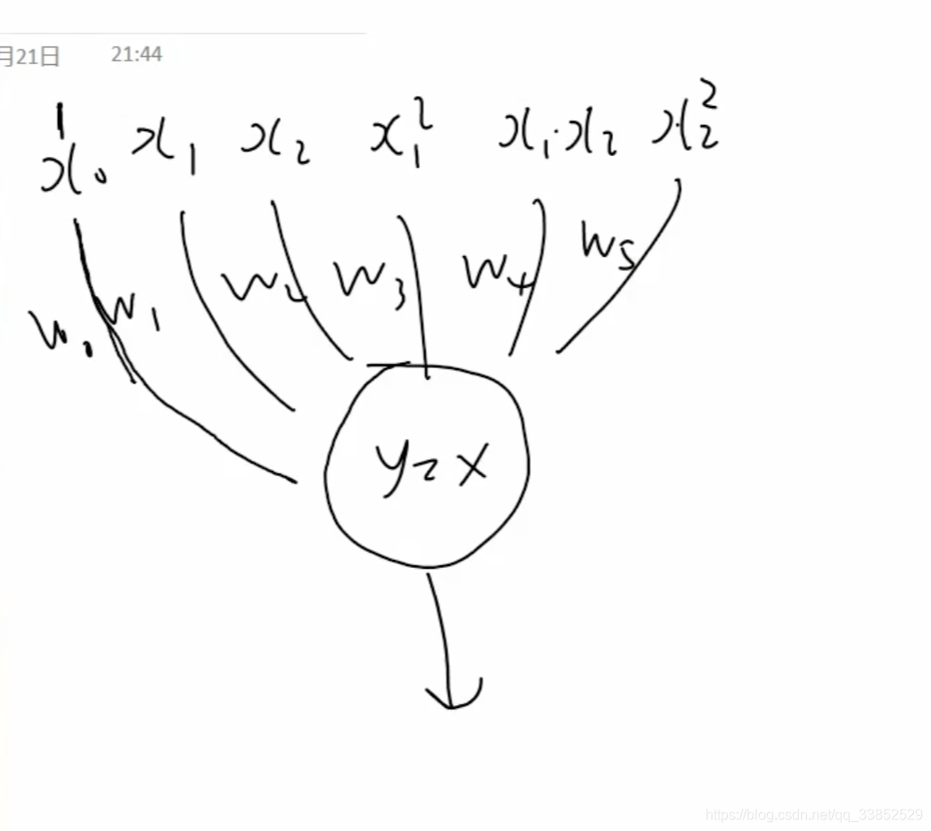
一、输入不能仅仅是x1和x2，而是 $x1,x1 \times x2,(x1)^{2},(x2)^{2}$ ,也就是引入了非线性的输入

线性神经网络的输入

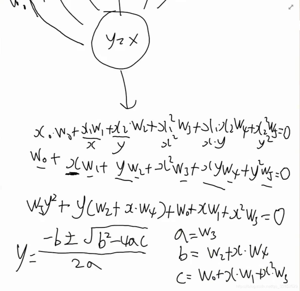
二、根据输出和输出激活函数（此时训练的输出激活函数是线性函数而不是sign函数）计算出输出

计算输出结果

三、完整python的代码


# coding: utf-8

# 微信公众号：深度学习与神经网络  
# Github：https://github.com/Qinbf  
# 优酷频道：http://i.youku.com/sdxxqbf  

# In[6]:

import numpy as np
import matplotlib.pyplot as plt


# In[7]:

#输入数据
X = np.array([[1,0,0,0,0,0],
              [1,0,1,0,0,1],
              [1,1,0,1,0,0],
              [1,1,1,1,1,1]])
#标签
Y = np.array([-1,1,1,-1])
#权值初始化，1行3列，取值范围-1到1
W = (np.random.random(6)-0.5)*2
print(W)
#学习率设置
lr = 0.11
#计算迭代次数
n = 0
#神经网络输出
O = 0

def update():
    global X,Y,W,lr,n
    n+=1
    O = np.dot(X,W.T)
    W_C = lr*((Y-O.T).dot(X))/int(X.shape[0])
    W = W + W_C


# In[10]:

for _ in range(100000):
    update()#更新权值
    #-0.1,0.1,0.2,-0.2
    #-1,1,1,-1


#正样本
x1 = [0,1]
y1 = [1,0]
#负样本
x2 = [0,1]
y2 = [0,1]

def calculate(x,root):
    a = W[5]
    b = W[2]+x*W[4]
    c = W[0]+x*W[1]+x*x*W[3]
    if root==1:
        return (-b+np.sqrt(b*b-4*a*c))/(2*a)
    if root==2:
        return (-b-np.sqrt(b*b-4*a*c))/(2*a)
    

xdata = np.linspace(-1,2)

plt.figure()

plt.plot(xdata,calculate(xdata,1),'r')
plt.plot(xdata,calculate(xdata,2),'r')

plt.plot(x1,y1,'bo')
plt.plot(x2,y2,'yo')
plt.show()

print(W)


# In[15]:

O = np.dot(X,W.T)
print(O)


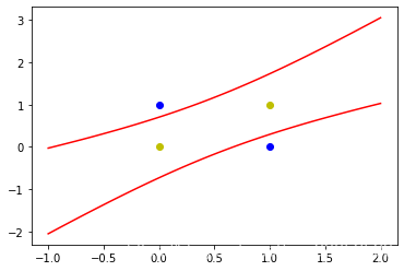
# In[ ]:

四、运行100000次后的图像

结果图像