深度学习 | 吴恩达深度学习课程 Week2

1 向量化VS非向量化实例

import numpy as np
a = np.array([1,2,3,4])
print(a)

[1 2 3 4]

知识点补充：

• np.random.rand函数 返回一个或一组服从**“0~1”均匀分布**的随机样本值。随机样本取值范围是[0,1)，不包括1
• np.random.randn函数 返回一个或一组服从标准正态分布的随机样本值。
• 参考：https://blog.youkuaiyun.com/qq_40130759/article/details/79535575

import time
# 先定义两个数组
a = np.random.rand(1000000) 
b = np.random.rand(1000000) 

# 向量化操作
t0 = time.time()
c = np.dot(a,b)
t1 = time.time()
print(c)
print('向量化所需时间为 %.4f ms' % ((t1-t0)*1000))

# 非向量化
t0 = time.time()
c = 0
for i in range(len(a)):
    c += a[i] * b[i]
t1 = time.time()
print(c)
print('非向量化（循环loop）所需时间为 %.4f ms' % ((t1-t0)*1000))

250238.1045275224
向量化所需时间为 0.9279 ms
250238.10452752237
非向量化（循环loop）所需时间为 402.1828 ms

结论：向量化的计算速度比非向量化快了接近400倍！

2 初始化很多变量为0时的向量化表示

dw1 = 0

dw2 = 0

dw3 = 0

…

dwn = 0

np.zeros((5,1))

array([[0.],
       [0.],
       [0.],
       [0.],
       [0.]])

3 Python中的广播

fruit = np.matrix([[56, 0, 4.4, 68],
                 [1.2, 104, 52, 8],
                 [1.8, 135, 99, 0.9]])
fruit

matrix([[ 56. ,   0. ,   4.4,  68. ],
        [  1.2, 104. ,  52. ,   8. ],
        [  1.8, 135. ,  99. ,   0.9]])

3.1 方法1

fruit / fruit.sum(axis=0) * 100# axis=0表示竖向求和！

matrix([[94.91525424,  0.        ,  2.83140283, 88.42652796],
        [ 2.03389831, 43.51464435, 33.46203346, 10.40312094],
        [ 3.05084746, 56.48535565, 63.70656371,  1.17035111]])

3.2 方法2

cal = fruit.sum(axis=0)
cal

matrix([[ 59. , 239. , 155.4,  76.9]])

100 * fruit / (cal.reshape(1,4))

matrix([[94.91525424,  0.        ,  2.83140283, 88.42652796],
        [ 2.03389831, 43.51464435, 33.46203346, 10.40312094],
        [ 3.05084746, 56.48535565, 63.70656371,  1.17035111]])

100 * fruit / cal

matrix([[94.91525424,  0.        ,  2.83140283, 88.42652796],
        [ 2.03389831, 43.51464435, 33.46203346, 10.40312094],
        [ 3.05084746, 56.48535565, 63.70656371,  1.17035111]])

3.3 其余例子

a = np.array([[1,2,3],[4,5,6]])
b = np.array([100,200,300])
a+b

array([[101, 202, 303],
       [104, 205, 306]])

4 Python中容易出错的点

a = np.random.randn(5)
print(a)

[-0.71991686 -0.66144438  0.18551096  1.28798856  0.92243471]

• 上面是数组
• rank为1的数组
• 不建议使用

print(a.shape)

(5,)

print(a.T)

[-0.71991686 -0.66144438  0.18551096  1.28798856  0.92243471]

print(np.dot(a, a.T))

3.500003614661412

总结：尽量避免(5,)这种结构形式

a = np.random.randn(5,1)
print(a)

[[ 1.71216331]
 [ 0.52272363]
 [-0.75470002]
 [-0.07638065]
 [ 1.10361583]]

• a.shpe = (5,1)

print(a.T)

[[ 1.71216331  0.52272363 -0.75470002 -0.07638065  1.10361583]]

• 上面是矩阵

print(np.dot(a, a.T))

[[ 2.9315032   0.89498822 -1.29216969 -0.13077615  1.88957054]
 [ 0.89498822  0.27323999 -0.39449954 -0.03992597  0.57688607]
 [-1.29216969 -0.39449954  0.56957213  0.05764448 -0.8328989 ]
 [-0.13077615 -0.03992597  0.05764448  0.005834   -0.0842949 ]
 [ 1.88957054  0.57688607 -0.8328989  -0.0842949   1.21796791]]

确认矩阵的维度，可以使用assert

assert(a.shape==(5,2))

---------------------------------------------------------------------------

AssertionError                            Traceback (most recent call last)

<ipython-input-51-280cb9b67a6c> in <module>()
----> 1 assert(a.shape==(5,2))


AssertionError: 

assert(a.shape==(5,1))

5 Week 2 Quiz - Neural Network Basics

1、What does a neuron compute?

[ ] A neuron computes an activation function followed by a linear function (z = Wx + b)

[✅] A neuron computes a linear function (z = Wx + b) followed by an activation function

[ ] A neuron computes a function g that scales the input x linearly (Wx + b)

[ ] A neuron computes the mean of all features before applying the output to an activation function

Note: The output of a neuron is a = g(Wx + b) where g is the activation function (sigmoid, tanh, ReLU, …).

解释：神经元计算的是什么，就是计算的线性表达式，然后外面套一层激活函数！
$$\sigma (w^{T}x+b)$$

3、Suppose img is a (32,32,3) array, representing a 32x32 image with 3 color channels red, green and blue. How do you reshape this into a column vector?

A = np.random.rand(32,32,3)
A

array([[[0.61840302, 0.84628931, 0.17072341],
        [0.02875052, 0.35218443, 0.18067854],
        [0.53842174, 0.0905776 , 0.64538035],
        ...,
        [0.86504037, 0.16503441, 0.58809624],
        [0.15577208, 0.90792988, 0.26518359],
        [0.14379626, 0.3932581 , 0.56879843]],

       [[0.77794977, 0.0157574 , 0.73827934],
        [0.49284295, 0.30152969, 0.94784409],
        [0.9894733 , 0.00746697, 0.92906519],
        ...,
        [0.58727335, 0.65692752, 0.88171581],
        [0.84406069, 0.65644595, 0.40225207],
        [0.33682128, 0.70572938, 0.82016853]],

       [[0.76552922, 0.6535839 , 0.3405907 ],
        [0.46168685, 0.93219971, 0.41885185],
        [0.49268255, 0.25078382, 0.83093396],
        ...,
        [0.1971106 , 0.21333168, 0.39811928],
        [0.22929499, 0.79545427, 0.73558373],
        [0.26466302, 0.61124282, 0.49819658]],

       ...,

       [[0.81421949, 0.51341299, 0.99480997],
        [0.16140379, 0.25647034, 0.88197708],
        [0.31393998, 0.08272694, 0.42572108],
        ...,
        [0.25752654, 0.24770792, 0.44660685],
        [0.37864687, 0.41302909, 0.29443527],
        [0.64505778, 0.12977772, 0.22643417]],

       [[0.01014001, 0.17776719, 0.96722298],
        [0.3321335 , 0.45471456, 0.77234341],
        [0.63661089, 0.21687891, 0.540193  ],
        ...,
        [0.98671685, 0.61813282, 0.72686287],
        [0.63619992, 0.5379135 , 0.23524182],
        [0.4870977 , 0.53408094, 0.59488148]],

       [[0.44804074, 0.03515261, 0.29183324],
        [0.65565814, 0.9698381 , 0.74386918],
        [0.5782844 , 0.90453468, 0.26510756],
        ...,
        [0.23110116, 0.21775663, 0.44895068],
        [0.65605225, 0.32334553, 0.43842636],
        [0.98404133, 0.57269513, 0.39178054]]])

A.reshape(32*32*3,1)

array([[0.61840302],
       [0.84628931],
       [0.17072341],
       ...,
       [0.98404133],
       [0.57269513],
       [0.39178054]])

4、Consider the two following random arrays “a” and “b”:

a = np.random.randn(2, 3) # a.shape = (2, 3)

b = np.random.randn(2, 1) # b.shape = (2, 1)

c = a + b

What will be the shape of “c”?

答案：根据Python广播，答案应该是 c.shape=(2,3)

a = np.random.randn(2, 3) 
b = np.random.randn(2, 1)
c = a + b
print(c.shape)

(2, 3)

5、Consider the two following random arrays “a” and “b”:

a = np.random.randn(2, 3) # a.shape = (2, 3)

b = np.random.randn(2, 1) # b.shape = (2, 1)

c = a * b

What will be the shape of “c”?

答案：根据Python广播，答案应该是 c.shape=(2,3)

a = np.random.randn(2, 3) 
b = np.random.randn(2, 1)
c = a * b # 对应元素相乘
print(a)
print(b)
print(c)
print(c.shape) 

[[-0.93462733  0.1371112   1.41004009]
 [ 0.92021926  0.01362638 -1.15927357]]
[[-0.38029658]
 [ 0.40306366]]
[[ 0.35543558 -0.05214292 -0.53623343]
 [ 0.37090694  0.0054923  -0.46726104]]
(2, 3)

6、Suppose you have n_x input features per example. Recall that X=[x^(1), x^(2)…x(m)]. What is the dimension of X?

n_x * m

7、Recall that np.dot(a,b) performs a matrix multiplication on a and b, whereas a*b performs an element-wise multiplication.Consider the two following random arrays “a” and “b”:

a = np.random.randn(12288, 150) # a.shape = (12288, 150)

b = np.random.randn(150, 45) # b.shape = (150, 45)

c = np.dot(a, b)

What is the shape of c?

答案：12288 * 45

a = np.random.randn(12288, 150) # a.shape = (12288, 150)
b = np.random.randn(150, 45) # b.shape = (150, 45)
c = np.dot(a, b)
print(c.shape)

(12288, 45)

知识点：

• np.dot代表矩阵相乘 符合乘法规则。对于二维矩阵，计算真正意义上的矩阵乘积，同线性代数中矩阵乘法的定义。对于一维矩阵，计算两者的内积（即对应元素相乘）。举例见下面
• x * y 或者 np.multiply() 则表示对应元素直接点乘！

import numpy as np

# 2-D array: 2 x 3 二维矩阵 符合线代中矩阵乘积
two_dim_matrix_one = np.array([[1, 2, 3], [4, 5, 6]])
# 2-D array: 3 x 2
two_dim_matrix_two = np.array([[1, 2], [3, 4], [5, 6]])

two_multi_res = np.dot(two_dim_matrix_one, two_dim_matrix_two)
print('two_multi_res: %s \n shape: %s' %(two_multi_res, two_multi_res.shape))

# 1-D array 一维矩阵 直接相乘
one_dim_vec_one = np.array([1, 2, 3])
one_dim_vec_two = np.array([4, 5, 6])
one_result_res = np.dot(one_dim_vec_one, one_dim_vec_two)
print('one_result_res: %s \n shape: %s' %(one_result_res, one_result_res.shape))

two_multi_res: [[22 28]
 [49 64]] 
 shape: (2, 2)
one_result_res: 32 
 shape: ()

import numpy as np

# 2-D array: 2 x 3
two_dim_matrix_one = np.array([[1, 2, 3], [4, 5, 6]])
another_two_dim_matrix_one = np.array([[7, 8, 9], [4, 7, 1]])

# 对应元素相乘 element-wise product
element_wise = two_dim_matrix_one * another_two_dim_matrix_one
print('element wise product: %s' %(element_wise))

# 对应元素相乘 element-wise product
element_wise_2 = np.multiply(two_dim_matrix_one, another_two_dim_matrix_one)
print('element wise product: %s' % (element_wise_2))

element wise product: [[ 7 16 27]
 [16 35  6]]
element wise product: [[ 7 16 27]
 [16 35  6]]

8、Consider the following code snippet:


# a.shape = (3,4)

# b.shape = (4,1)

for i in range(3):

    for j in range(4):
    
        c[i][j] = a[i][j] + b[j]

# How do you vectorize this?

a = np.random.rand(3,4)
print(a)
b = np.random.rand(4,1)
print(b)
c = a + b.T
print(c.shape)
print(c)

[[0.95093896 0.967598   0.54171538 0.99492865]
 [0.12774542 0.42832552 0.189236   0.22077887]
 [0.55143021 0.95713185 0.91650609 0.29207027]]
[[0.98992572]
 [0.06027574]
 [0.4486389 ]
 [0.51615222]]
(3, 4)
[[1.94086468 1.02787374 0.99035428 1.51108087]
 [1.11767114 0.48860126 0.6378749  0.7369311 ]
 [1.54135593 1.01740759 1.36514499 0.80822249]]

9、Consider the following code:

a = np.random.randn(3, 3)

b = np.random.randn(3, 1)

c = a * b

What will be c?

c.shape = (3,3) 对应点乘

a = np.random.randn(3, 3)
print(a)
b = np.random.randn(3, 1)
print(b)
c = a * b
print(c)

[[-1.05691807  0.30545018  0.36232241]
 [ 0.0839955   0.9658852   0.28260075]
 [ 1.19398702  0.39351986 -0.93235503]]
[[-0.29285184]
 [ 1.58090438]
 [ 0.36897749]]
[[ 0.3095204  -0.08945165 -0.10610679]
 [ 0.13278885  1.52697214  0.44676477]
 [ 0.44055433  0.14519997 -0.34401801]]

6 编程作业：具有神经网络思维的Logistic回归

我们要做的事是搭建一个能够【识别猫】 的简单的神经网络。

总结：

• 针对图片的三维数据，进行一个压缩，变成一维！
• 压缩后的数据表现就是按行进行拼接，比如64×64×3 表示的是 64×64维的图片有3张！一张图片拼接的结果就是64×64，相当于正方形第一行不变，剩余的63行都横着拼接在第一行后面，即相当于64×64个特征维度了，最后再乘以3！
• 上面这样处理的目的是数据变成了二维，即样本量×维度，就可以用普通的逻辑回归来处理了！
• 后续应该可以用神经网络比如CNN来进行处理！

import numpy as np
import matplotlib.pyplot as plt
import h5py # 是与H5文件中存储的数据集进行交互的常用软件包。
from lr_utils import load_dataset # 在本文的资料包里，一个加载资料包里面的数据的简单功能的库。

lr_utils.py的代码

import numpy as np
import h5py
    
    
def load_dataset():
    train_dataset = h5py.File('datasets/train_catvnoncat.h5', "r")
    train_set_x_orig = np.array(train_dataset["train_set_x"][:]) # your train set features
    train_set_y_orig = np.array(train_dataset["train_set_y"][:]) # your train set labels

    test_dataset = h5py.File('datasets/test_catvnoncat.h5', "r")
    test_set_x_orig = np.array(test_dataset["test_set_x"][:]) # your test set features
    test_set_y_orig = np.array(test_dataset["test_set_y"][:]) # your test set labels

    classes = np.array(test_dataset["list_classes"][:]) # the list of classes
    
    train_set_y_orig = train_set_y_orig.reshape((1, train_set_y_orig.shape[0]))
    test_set_y_orig = test_set_y_orig.reshape((1, test_set_y_orig.shape[0]))
    
    return train_set_x_orig, train_set_y_orig, test_set_x_orig, test_set_y_orig, classes

• train_set_x_orig ：保存的是训练集里面的图像数据（本训练集有209张64x64的图像）。
• train_set_y_orig ：保存的是训练集的图像对应的分类值（【0 | 1】，0表示不是猫，1表示是猫）。
• test_set_x_orig ：保存的是测试集里面的图像数据（本训练集有50张64x64的图像）。
• test_set_y_orig ： 保存的是测试集的图像对应的分类值（【0 | 1】，0表示不是猫，1表示是猫）。
• classes ： 保存的是以bytes类型保存的两个字符串数据，数据为：[b’non-cat’ b’cat’]。

6.1 载入数据

train_set_x_orig , train_set_y , test_set_x_orig , test_set_y , classes = load_dataset()
print(train_set_x_orig.shape , train_set_y.shape , test_set_x_orig.shape , test_set_y.shape , classes.shape)

(209, 64, 64, 3) (1, 209) (50, 64, 64, 3) (1, 50) (2,)

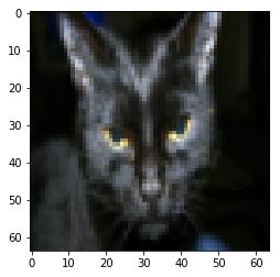
6.2 看一个示例

index = 25
plt.imshow(train_set_x_orig[index])
print("train_set_y=" + str(train_set_y)) # 看一下训练集里面的标签是什么样的。

train_set_y=[[0 0 1 0 0 0 0 1 0 0 0 1 0 1 1 0 0 0 0 1 0 0 0 0 1 1 0 1 0 1 0 0 0 0 0 0
  0 0 1 0 0 1 1 0 0 0 0 1 0 0 1 0 0 0 1 0 1 1 0 1 1 1 0 0 0 0 0 0 1 0 0 1
  0 0 0 0 0 0 0 0 0 0 0 1 1 0 0 0 1 0 0 0 1 1 1 0 0 1 0 0 0 0 1 0 1 0 1 1
  1 1 1 1 0 0 0 0 0 1 0 0 0 1 0 0 1 0 1 0 1 1 0 0 0 1 1 1 1 1 0 0 0 0 1 0
  1 1 1 0 1 1 0 0 0 1 0 0 1 0 0 0 0 0 1 0 1 0 1 0 0 1 1 1 0 0 1 1 0 1 0 1
  0 0 0 0 0 1 0 0 1 0 0 0 1 0 0 0 0 1 0 0 1 0 0 0 0 0 0 0 0]]

train_set_y[0][25] # 表示是猫

1

print(train_set_y[:,index])
print(np.squeeze(train_set_y[:,index]))

[1]
1

print(classes)
print(classes[1])
print(classes[0])

[b'non-cat' b'cat']
b'cat'
b'non-cat'

#打印出当前的训练标签值
#使用np.squeeze的目的是压缩维度，【未压缩】train_set_y[:,index]的值为[1] , 【压缩后】np.squeeze(train_set_y[:,index])的值为1
#print("【使用np.squeeze：" + str(np.squeeze(train_set_y[:,index])) + "，不使用np.squeeze： " + str(train_set_y[:,index]) + "】")
#只有压缩后的值才能进行解码操作
print("y=" + str(train_set_y[:,index]) + ", it's a " + classes[np.squeeze(train_set_y[:,index])].decode("utf-8") + "' picture")

y=[1], it's a cat' picture

6.3 查看图片具体情况

print(train_set_x_orig.shape[0])
print(train_set_x_orig.shape[1])
print(train_set_x_orig.shape[2])
print(train_set_x_orig.shape[3])

209
64
64
3

m_train = train_set_y.shape[1] # 训练集里图片的数量。
m_test = test_set_y.shape[1] # 测试集里图片的数量。
num_px = train_set_x_orig.shape[1] # 训练、测试集里面的图片的宽度和高度（均为64x64）。

#现在看一看我们加载的东西的具体情况
print ("训练集的数量: m_train = " + str(m_train))
print ("测试集的数量 : m_test = " + str(m_test))
print ("每张图片的宽/高 : num_px = " + str(num_px))
print ("每张图片的大小 : (" + str(num_px) + ", " + str(num_px) + ", 3)")
print ("训练集_图片的维数 : " + str(train_set_x_orig.shape))
print ("训练集_标签的维数 : " + str(train_set_y.shape))
print ("测试集_图片的维数: " + str(test_set_x_orig.shape))
print ("测试集_标签的维数: " + str(test_set_y.shape))

训练集的数量: m_train = 209
测试集的数量 : m_test = 50
每张图片的宽/高 : num_px = 64
每张图片的大小 : (64, 64, 3)
训练集_图片的维数 : (209, 64, 64, 3)
训练集_标签的维数 : (1, 209)
测试集_图片的维数: (50, 64, 64, 3)
测试集_标签的维数: (1, 50)

6.4 降维处理

• 为了方便，我们要把维度为（64，64，3）的numpy数组重新构造为（64 x 64 x 3，1）的数组，
• 要乘以3的原因是每张图片是由64x64像素构成的，而每个像素点由（R，G，B）三原色构成的，所以要乘以3。
• 在此之后，我们的训练和测试数据集是一个numpy数组，【每列代表一个平坦的图像】 ，应该有m_train和m_test列。

当你想将形状（a，b，c，d）的矩阵X平铺成形状（b * c * d，a）的矩阵X_flatten时，可以使用以下代码：

6.4.1 Python实现

#X_flatten = X.reshape(X.shape [0]，-1).T ＃X.T是X的转置
#将训练集的维度降低并转置。
train_set_x_flatten  = train_set_x_orig.reshape(train_set_x_orig.shape[0],-1).T # 把209单独拿出来 其余相乘作为一个新维度
print(train_set_x_flatten.shape)
#将测试集的维度降低并转置。
test_set_x_flatten = test_set_x_orig.reshape(test_set_x_orig.shape[0], -1).T 
print(test_set_x_flatten.shape)

(12288, 209)
(12288, 50)

6.4.2 测试reshape(n,-1)函数

作用：把原始数据的n保留 其余维度全乘起来！起到降维的作用

a = np.random.rand(2,3,3,4)
print(a.shape)
a

(2, 3, 3, 4)





array([[[[0.46361438, 0.33743967, 0.40810738, 0.1522352 ],
         [0.85740791, 0.78962262, 0.58285323, 0.89033907],
         [0.7330014 , 0.35565149, 0.77499978, 0.0259401 ]],

        [[0.4214553 , 0.52551294, 0.41082593, 0.77709762],
         [0.55332002, 0.40664621, 0.01146762, 0.52825587],
         [0.03558865, 0.50706837, 0.99895553, 0.00286304]],

        [[0.95963041, 0.78539995, 0.23660636, 0.71023432],
         [0.07496047, 0.93362626, 0.22808421, 0.03347676],
         [0.28634181, 0.61336991, 0.50548084, 0.17436676]]],


       [[[0.09105066, 0.32129605, 0.93116884, 0.62145194],
         [0.0072716 , 0.96740441, 0.936825  , 0.37791679],
         [0.49590378, 0.55241354, 0.39232398, 0.44347483]],

        [[0.40645334, 0.45936483, 0.1692183 , 0.05136581],
         [0.12079697, 0.89790619, 0.98934628, 0.33832818],
         [0.94331331, 0.67024107, 0.42825149, 0.45080149]],

        [[0.12879168, 0.0225791 , 0.11612455, 0.67521729],
         [0.8141249 , 0.15929005, 0.72741135, 0.06385646],
         [0.88465748, 0.15984815, 0.68050255, 0.05219639]]]])

b = a.reshape(2,-1) # 即作用是把3单独拿出来 后面全部乘起来作为一个维度！具体就是把数字拼起来！
print(b.shape)
b

(2, 36)





array([[0.46361438, 0.33743967, 0.40810738, 0.1522352 , 0.85740791,
        0.78962262, 0.58285323, 0.89033907, 0.7330014 , 0.35565149,
        0.77499978, 0.0259401 , 0.4214553 , 0.52551294, 0.41082593,
        0.77709762, 0.55332002, 0.40664621, 0.01146762, 0.52825587,
        0.03558865, 0.50706837, 0.99895553, 0.00286304, 0.95963041,
        0.78539995, 0.23660636, 0.71023432, 0.07496047, 0.93362626,
        0.22808421, 0.03347676, 0.28634181, 0.61336991, 0.50548084,
        0.17436676],
       [0.09105066, 0.32129605, 0.93116884, 0.62145194, 0.0072716 ,
        0.96740441, 0.936825  , 0.37791679, 0.49590378, 0.55241354,
        0.39232398, 0.44347483, 0.40645334, 0.45936483, 0.1692183 ,
        0.05136581, 0.12079697, 0.89790619, 0.98934628, 0.33832818,
        0.94331331, 0.67024107, 0.42825149, 0.45080149, 0.12879168,
        0.0225791 , 0.11612455, 0.67521729, 0.8141249 , 0.15929005,
        0.72741135, 0.06385646, 0.88465748, 0.15984815, 0.68050255,
        0.05219639]])

print ("训练集降维最后的维度： " + str(train_set_x_flatten.shape))
print ("训练集_标签的维数 : " + str(train_set_y.shape))
print ("测试集降维之后的维度: " + str(test_set_x_flatten.shape))
print ("测试集_标签的维数 : " + str(test_set_y.shape))

训练集降维最后的维度： (12288, 209)
训练集_标签的维数 : (1, 209)
测试集降维之后的维度: (12288, 50)
测试集_标签的维数 : (1, 50)

6.5 标准化

• 一般的标准化方法不适用于此处，因为图片的数据为RGB，范围均在0-255之间！
• 对于图片数据集，它更简单，更方便，几乎可以将数据集的每一行除以255（像素通道的最大值），因为在RGB中不存在比255大的数据，所以我们可以放心的除以255，让标准化的数据位于[0,1]之间

train_set_x = train_set_x_flatten / 255
test_set_x = test_set_x_flatten / 255

6.6 主要步骤

建立神经网络的主要步骤是：

1. 定义模型结构（例如输入特征的数量）

2. 初始化模型的参数

3. 循环：

   3.1 计算当前损失（正向传播）

   3.2 计算当前梯度（反向传播）

   3.3 更新参数（梯度下降）

4. 预测

6.6.1 定义激活函数

def sigmoid(z):
    """
    参数：
        z  - 任何大小的标量或numpy数组。

    返回：
        s  -  sigmoid（z）
    """
    s = 1 / (1 + np.exp(-z))
    return s

# 测试sigmoid()
print("====================测试sigmoid====================")
print ("sigmoid(0) = ", (sigmoid(0)))
print ("sigmoid(9.2) = ", (sigmoid(9.2)))

====================测试sigmoid====================
sigmoid(0) =  0.5
sigmoid(9.2) =  0.9998989708060922

6.6.2 初始化参数w b

def initialize_with_zeros(dim):
    """
        此函数为w创建一个维度为（dim，1）的0向量，并将b初始化为0。

        参数：
            dim  - 我们想要的w矢量的大小（或者这种情况下的参数数量）
            dim和数据集特征的维度保持一致！比如有10个变量，就应该有10个变量对应的系数！
            所以应该是train的shape之一！

        返回：
            w  - 维度为（dim，1）的初始化向量。
            b  - 初始化的标量（对应于偏差）
    """
    w = np.zeros(shape = (dim,1))
    b = 0
    # 使用断言来确保我要的数据是正确的
    assert(w.shape == (dim, 1)) # w的维度是(dim,1)
    assert(isinstance(b, float) or isinstance(b, int)) # b的类型是float或者是int

    return (w , b)

6.6.3 前向后向传播

• 初始化参数的函数已经构建好了，现在就可以执行“前向”和“后向”传播步骤来学习参数。
• 我们现在要实现一个计算成本函数及其渐变的函数propagate（）。
• 其实就是参数学习过程的前奏，你得去定义出损失函数+参数w的导数+参数b的导数

def propagate(w, b, X, Y):
    """
    实现前向和后向传播的成本函数及其梯度。
    参数：
        w  - 权重，大小不等的数组（num_px * num_px * 3，1）
        b  - 偏差，一个标量
        X  - 矩阵类型为（num_px * num_px * 3，训练数量）
        Y  - 真正的“标签”矢量（如果非猫则为0，如果是猫则为1），矩阵维度为(1,训练数据数量)

    返回：
        cost- 逻辑回归的负对数似然成本
        dw  - 相对于w的损失梯度，因此与w相同的形状
        db  - 相对于b的损失梯度，因此与b的形状相同
    """
    m = X.shape[1] # 数据集样本量

    # 正向传播-计算激活值+总损失函数值
    A = sigmoid(np.dot(w.T,X) + b) # 计算激活值，请参考公式2。
    cost = (- 1 / m) * np.sum(Y * np.log(A) + (1 - Y) * (np.log(1 - A))) # 计算总成本，请参考公式3和4。

    #反向传播-计算梯度 dw db
    dw = (1 / m) * np.dot(X, (A - Y).T) # 请参考视频中的偏导公式。 A-Y都是横着减 需要立起来 即 m * 1
    db = (1 / m) * np.sum(A - Y) # 请参考视频中的偏导公式。

    # 使用断言确保我的数据是正确的
    assert(dw.shape == w.shape)
    assert(db.dtype == float)
    cost = np.squeeze(cost)
    assert(cost.shape == ())

    # 创建一个字典，把dw和db保存起来。
    grads = {
                "dw": dw,
                "db": db
             }
    return (grads , cost)

#测试一下propagate
print("====================测试propagate====================")
#初始化一些参数
w, b, X, Y = np.array([[1], [2]]), 2, np.array([[1,2], [3,4]]), np.array([[1, 0]])
grads, cost = propagate(w, b, X, Y)
print ("dw = " + str(grads["dw"]))
print ("db = " + str(grads["db"]))
print ("cost = " + str(cost))

====================测试propagate====================
dw = [[0.99993216]
 [1.99980262]]
db = 0.49993523062470574
cost = 6.000064773192205

dw.shape

(1, 2)

6.6.4 更新参数

def optimize(w , b , X , Y , num_iterations , learning_rate , print_cost = False):
    """
    此函数通过运行梯度下降算法来优化w和b

    参数：
        w  - 权重，大小不等的数组（num_px * num_px * 3，1）
        b  - 偏差，一个标量
        X  - 维度为（num_px * num_px * 3，训练数据的数量）的数组。
        Y  - 真正的“标签”矢量（如果非猫则为0，如果是猫则为1），矩阵维度为(1,训练数据的数量)
        num_iterations  - 优化循环的迭代次数
        learning_rate  - 梯度下降更新规则的学习率
        print_cost  - 每100步打印一次损失值

    返回：
        params  - 包含权重w和偏差b的字典
        grads  - 包含权重和偏差相对于成本函数的梯度的字典
        costs - 优化期间计算的所有成本列表，将用于绘制学习曲线。

    提示：
    我们需要写下两个步骤并遍历它们：
        1）计算当前参数的成本和梯度，使用propagate（）。
        2）使用w和b的梯度下降法则更新参数。
    """

    costs = []

    for i in range(num_iterations):

        grads, cost = propagate(w, b, X, Y)

        dw = grads["dw"]
        db = grads["db"]

        w = w - learning_rate * dw
        b = b - learning_rate * db

        #记录成本
        if i % 100 == 0:
            costs.append(cost)
        #打印成本数据
        if (print_cost) and (i % 100 == 0):
            print("迭代的次数: %i ， 误差值： %f" % (i,cost))

    params  = {
                "w" : w,
                "b" : b }
    grads = {
            "dw": dw,
            "db": db } 
    return (params , grads , costs)

#测试optimize
print("====================测试optimize====================")
w, b, X, Y = np.array([[1], [2]]), 2, np.array([[1,2], [3,4]]), np.array([[1, 0]])
params , grads , costs = optimize(w , b , X , Y , num_iterations=100 , learning_rate = 0.009 , print_cost = False)
print ("w = " + str(params["w"]))
print ("b = " + str(params["b"]))
print ("dw = " + str(grads["dw"]))
print ("db = " + str(grads["db"]))

====================测试optimize====================
w = [[0.1124579 ]
 [0.23106775]]
b = 1.5593049248448891
dw = [[0.90158428]
 [1.76250842]]
db = 0.4304620716786828

6.6.5 预测

两步：

• 先计算激活后的预测值 $$A=\hat{Y}=\sigma (w^{T}x+b)$$
• 然后根据这个结果将实例判别为0（A<0.5）或者1（A>0.5）

def predict(w , b , X ):
    """
    使用学习逻辑回归参数logistic （w，b）预测标签是0还是1，

    参数：
        w  - 权重，大小不等的数组（num_px * num_px * 3，1）
        b  - 偏差，一个标量
        X  - 维度为（num_px * num_px * 3，训练数据的数量）的数据

    返回：
        Y_prediction  - 包含X中所有图片的所有预测【0 | 1】的一个numpy数组（向量）

    """

    m  = X.shape[1] #图片的数量
    Y_prediction = np.zeros((1,m)) 
    w = w.reshape(X.shape[0],1)

    #预测猫在图片中出现的概率
    A = sigmoid(np.dot(w.T , X) + b)
    for i in range(A.shape[1]):
        #将概率a [0，i]转换为实际预测p [0，i]
        Y_prediction[0,i] = 1 if A[0,i] > 0.5 else 0
    #使用断言
    assert(Y_prediction.shape == (1,m))

    return Y_prediction

#测试predict
print("====================测试predict====================")
w, b, X, Y = np.array([[1], [2]]), 2, np.array([[1,2], [3,4]]), np.array([[1, 0]])
print("predictions = " + str(predict(w, b, X)))

====================测试predict====================
predictions = [[1. 1.]]

6.6.6 汇总函数

def model(X_train , Y_train , X_test , Y_test , num_iterations = 2000 , learning_rate = 0.5 , print_cost = False):
    """
    通过调用之前实现的函数来构建逻辑回归模型

    参数：
        X_train  - numpy的数组,维度为（num_px * num_px * 3，m_train）的训练集
        Y_train  - numpy的数组,维度为（1，m_train）（矢量）的训练标签集
        X_test   - numpy的数组,维度为（num_px * num_px * 3，m_test）的测试集
        Y_test   - numpy的数组,维度为（1，m_test）的（向量）的测试标签集
        num_iterations  - 表示用于优化参数的迭代次数的超参数
        learning_rate  - 表示optimize（）更新规则中使用的学习速率的超参数
        print_cost  - 设置为true以每100次迭代打印成本

    返回：
        d  - 包含有关模型信息的字典。
    """
    w , b = initialize_with_zeros(X_train.shape[0])

    parameters , grads , costs = optimize(w , b , X_train , Y_train,num_iterations , learning_rate , print_cost)

    #从字典“参数”中检索参数w和b
    w , b = parameters["w"] , parameters["b"]

    #预测测试/训练集的例子
    Y_prediction_test = predict(w , b, X_test)
    Y_prediction_train = predict(w , b, X_train)

    #打印训练后的准确性
    print("训练集准确性："  , format(100 - np.mean(np.abs(Y_prediction_train - Y_train)) * 100) ,"%")
    print("测试集准确性："  , format(100 - np.mean(np.abs(Y_prediction_test - Y_test)) * 100) ,"%")

    d = {
            "costs" : costs,
            "Y_prediction_test" : Y_prediction_test,
            "Y_prediciton_train" : Y_prediction_train,
            "w" : w,
            "b" : b,
            "learning_rate" : learning_rate,
            "num_iterations" : num_iterations }
    return d

print("====================测试model====================")     
#这里加载的是真实的数据，请参见上面的代码部分。
d = model(train_set_x, train_set_y, test_set_x, test_set_y, num_iterations = 2000, learning_rate = 0.005, print_cost = True)

====================测试model====================
迭代的次数: 0 ， 误差值： 0.693147
迭代的次数: 100 ， 误差值： 0.584508
迭代的次数: 200 ， 误差值： 0.466949
迭代的次数: 300 ， 误差值： 0.376007
迭代的次数: 400 ， 误差值： 0.331463
迭代的次数: 500 ， 误差值： 0.303273
迭代的次数: 600 ， 误差值： 0.279880
迭代的次数: 700 ， 误差值： 0.260042
迭代的次数: 800 ， 误差值： 0.242941
迭代的次数: 900 ， 误差值： 0.228004
迭代的次数: 1000 ， 误差值： 0.214820
迭代的次数: 1100 ， 误差值： 0.203078
迭代的次数: 1200 ， 误差值： 0.192544
迭代的次数: 1300 ， 误差值： 0.183033
迭代的次数: 1400 ， 误差值： 0.174399
迭代的次数: 1500 ， 误差值： 0.166521
迭代的次数: 1600 ， 误差值： 0.159305
迭代的次数: 1700 ， 误差值： 0.152667
迭代的次数: 1800 ， 误差值： 0.146542
迭代的次数: 1900 ， 误差值： 0.140872
训练集准确性： 99.04306220095694 %
测试集准确性： 70.0 %

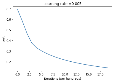
6.6.7 绘制损失函数下降曲线图

#绘制图
costs = np.squeeze(d['costs'])
plt.plot(costs)
plt.ylabel('cost')
plt.xlabel('iterations (per hundreds)')
plt.title("Learning rate =" + str(d["learning_rate"]))
plt.show()

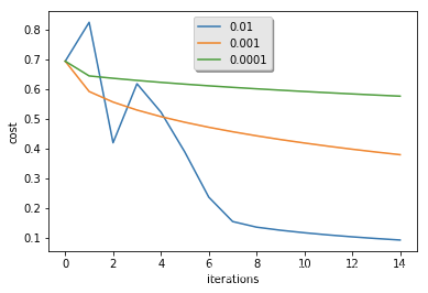
6.6.8 改变学习率看预测效果

learning_rates = [0.01, 0.001, 0.0001]
models = {}
for i in learning_rates:
    print ("learning rate is: " + str(i))
    models[str(i)] = model(train_set_x, train_set_y, test_set_x, test_set_y, num_iterations = 1500, learning_rate = i, print_cost = False)
    print ('\n' + "-------------------------------------------------------" + '\n')

for i in learning_rates:
    plt.plot(np.squeeze(models[str(i)]["costs"]), label= str(models[str(i)]["learning_rate"]))

plt.ylabel('cost')
plt.xlabel('iterations')

legend = plt.legend(loc='upper center', shadow=True)
frame = legend.get_frame()
frame.set_facecolor('0.90')
plt.show()

learning rate is: 0.01
训练集准确性： 99.52153110047847 %
测试集准确性： 68.0 %

-------------------------------------------------------

learning rate is: 0.001
训练集准确性： 88.99521531100478 %
测试集准确性： 64.0 %

-------------------------------------------------------

learning rate is: 0.0001
训练集准确性： 68.42105263157895 %
测试集准确性： 36.0 %

-------------------------------------------------------

6.7 Sklearn实现

print(train_set_x.shape, train_set_y.shape, test_set_x.shape, test_set_y.shape)

(12288, 209) (1, 209) (12288, 50) (1, 50)

train_set_x

array([[0.06666667, 0.76862745, 0.32156863, ..., 0.56078431, 0.08627451,
        0.03137255],
       [0.12156863, 0.75294118, 0.27843137, ..., 0.60784314, 0.09411765,
        0.10980392],
       [0.21960784, 0.74509804, 0.26666667, ..., 0.64705882, 0.09019608,
        0.20784314],
       ...,
       [0.        , 0.32156863, 0.54117647, ..., 0.33333333, 0.01568627,
        0.        ],
       [0.        , 0.31372549, 0.55294118, ..., 0.41960784, 0.01960784,
        0.        ],
       [0.        , 0.31764706, 0.55686275, ..., 0.58431373, 0.        ,
        0.        ]])

train_set_y

array([[0, 0, 1, 0, 0, 0, 0, 1, 0, 0, 0, 1, 0, 1, 1, 0, 0, 0, 0, 1, 0, 0,
        0, 0, 1, 1, 0, 1, 0, 1, 0, 0, 0, 0, 0, 0, 0, 0, 1, 0, 0, 1, 1, 0,
        0, 0, 0, 1, 0, 0, 1, 0, 0, 0, 1, 0, 1, 1, 0, 1, 1, 1, 0, 0, 0, 0,
        0, 0, 1, 0, 0, 1, 0, 0, 0, 0, 0, 0, 0, 0, 0, 0, 0, 1, 1, 0, 0, 0,
        1, 0, 0, 0, 1, 1, 1, 0, 0, 1, 0, 0, 0, 0, 1, 0, 1, 0, 1, 1, 1, 1,
        1, 1, 0, 0, 0, 0, 0, 1, 0, 0, 0, 1, 0, 0, 1, 0, 1, 0, 1, 1, 0, 0,
        0, 1, 1, 1, 1, 1, 0, 0, 0, 0, 1, 0, 1, 1, 1, 0, 1, 1, 0, 0, 0, 1,
        0, 0, 1, 0, 0, 0, 0, 0, 1, 0, 1, 0, 1, 0, 0, 1, 1, 1, 0, 0, 1, 1,
        0, 1, 0, 1, 0, 0, 0, 0, 0, 1, 0, 0, 1, 0, 0, 0, 1, 0, 0, 0, 0, 1,
        0, 0, 1, 0, 0, 0, 0, 0, 0, 0, 0]])

from sklearn.linear_model import LogisticRegression
from sklearn import metrics
from sklearn.metrics import roc_auc_score, classification_report, confusion_matrix
lr = LogisticRegression()
lr.fit(train_set_x.T, train_set_y.T)
pre = lr.predict(test_set_x.T)
print(metrics.roc_auc_score(test_set_y.T, pre))
print(classification_report(test_set_y.T, pre))
print(confusion_matrix(test_set_y.T, pre))

/Users/apple/anaconda3/lib/python3.6/site-packages/sklearn/linear_model/logistic.py:433: FutureWarning: Default solver will be changed to 'lbfgs' in 0.22. Specify a solver to silence this warning.
  FutureWarning)
/Users/apple/anaconda3/lib/python3.6/site-packages/sklearn/utils/validation.py:761: DataConversionWarning: A column-vector y was passed when a 1d array was expected. Please change the shape of y to (n_samples, ), for example using ravel().
  y = column_or_1d(y, warn=True)


0.7308377896613191
              precision    recall  f1-score   support

           0       0.57      0.76      0.65        17
           1       0.85      0.70      0.77        33

   micro avg       0.72      0.72      0.72        50
   macro avg       0.71      0.73      0.71        50
weighted avg       0.75      0.72      0.73        50

[[13  4]
 [10 23]]

pre

array([1, 1, 1, 1, 1, 0, 0, 1, 1, 1, 0, 0, 1, 1, 0, 1, 0, 1, 0, 0, 1, 0,
       0, 1, 0, 1, 1, 0, 0, 1, 0, 1, 1, 1, 0, 0, 0, 1, 0, 0, 1, 0, 1, 0,
       1, 1, 0, 1, 1, 0])

7 参考

• https://blog.youkuaiyun.com/u012609509/article/details/70230204
• https://blog.youkuaiyun.com/qq_40130759/article/details/79535575
• https://blog.youkuaiyun.com/u013733326/article/details/79865858
• https://blog.youkuaiyun.com/u013733326/article/details/79639509#commentBox
• http://www.ai-start.com/dl2017/