李沐pytorch学习-经典CNN的原理及代码实现

原创已于 2023-10-10 11:09:05 修改 · 898 阅读

4 ·

CC 4.0 BY-SA版权

文章标签：

#pytorch #学习 #cnn

于 2023-08-21 11:24:23 首次发布

深度学习基础知识专栏收录该内容

10 篇文章

订阅专栏

一、LeNet

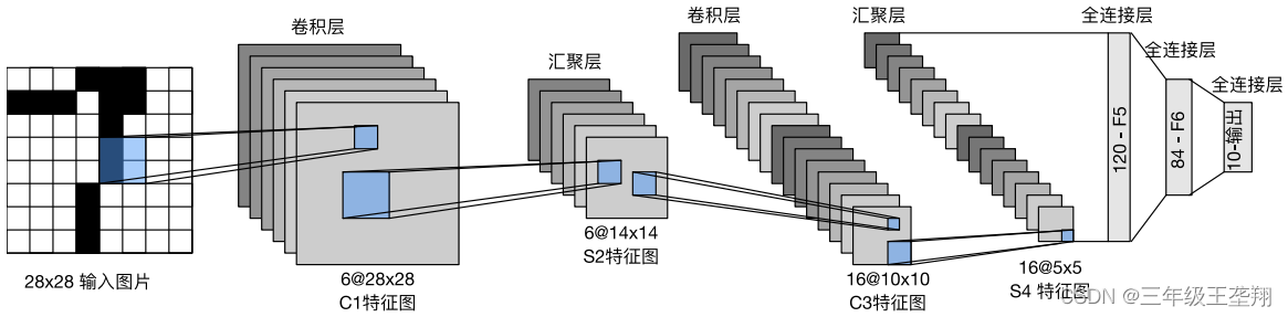
1.1 模型结构

LeNet结构如图1所示，汇聚层即池化层，这里池化Stride（步幅）与池化层长宽一致，因此使得池化后大小减半。

1.2 代码实现

代码实现如下：

import torch
from torch import nn
from d2l import torch as d2l

net = nn.Sequential(
    nn.Conv2d(1, 6, kernel_size=5, padding=2), nn.Sigmoid(),
    nn.AvgPool2d(kernel_size=2, stride=2),
    nn.Conv2d(6, 16, kernel_size=5), nn.Sigmoid(),
    nn.AvgPool2d(kernel_size=2, stride=2),
    nn.Flatten(),
    nn.Linear(16 * 5 * 5, 120), nn.Sigmoid(),
    nn.Linear(120, 84), nn.Sigmoid(),
    nn.Linear(84, 10))

        nn.Sequential 即表示把括号里的层按序排起来，代码与每层的对应关系如图2所示。

        nn.Flatten() 作用是将16@5×5的汇聚层展平程1维向量，作为全连接层的输入，因此不对应图中的某层。

        nn.Conv2d(1, 6, kernel_size=5, padding=2) 为卷积层，表示输入的通道数为1，输出的通道数为6，直观表达是经过该层后数据变“厚”了，卷积核大小为5×5，上下左右均填充2行（填充0）。nn.Sigmoid()表示该层的激活函数为Sigmoid。

        nn.AvgPool2d(kernel_size=2, stride=2) 表示平均池化，池化层大小为2×2，步幅为2。

        nn.Conv2d(6, 16, kernel_size=5), nn.Sigmoid() 为卷积层，四周无填充，激活函数为Sigmoid。

        nn.AvgPool2d(kernel_size=2, stride=2) 为平均池化层。

        nn.Linear(16 * 5 * 5, 120), nn.Sigmoid() 为线性全连接层，输入层神经元数为16×5×5，输出层神经元数为120，无隐含层，激活函数为Sigmoid。

        nn.Linear(120, 84), nn.Sigmoid() 为线性全连接层，输入层神经元数为120，输出层神经元数为84，无隐含层，激活函数为Sigmoid。

        nn.Linear(84, 10) 为线性全连接层，输入层神经元数为84，输出层神经元数为10，无隐含层，无激活函数。

1.3 检查模型

查看输出层的名及Size。

import torch
from torch import nn
from d2l import torch as d2l

net = nn.Sequential(
    nn.Conv2d(1, 6, kernel_size=5, padding=2), nn.Sigmoid(),
    nn.AvgPool2d(kernel_size=2, stride=2),
    nn.Conv2d(6, 16, kernel_size=5), nn.Sigmoid(),
    nn.AvgPool2d(kernel_size=2, stride=2),
    nn.Flatten(),
    nn.Linear(16 * 5 * 5, 120), nn.Sigmoid(),
    nn.Linear(120, 84), nn.Sigmoid(),
    nn.Linear(84, 10))

X = torch.rand(size=(1, 1, 28, 28), dtype=torch.float32)
for layer in net:
    X = layer(X)
    print(layer.__class__.__name__,'output shape: \t',X.shape)

# 输出如下：
Conv2d output shape: torch.Size([1, 6, 28, 28])
Sigmoid output shape: torch.Size([1, 6, 28, 28])
AvgPool2d output shape: torch.Size([1, 6, 14, 14])
Conv2d output shape: torch.Size([1, 16, 10, 10])
Sigmoid output shape: torch.Size([1, 16, 10, 10])
AvgPool2d output shape: torch.Size([1, 16, 5, 5])
Flatten output shape: torch.Size([1, 400])

1.4 训练模型

import torch
from torch import nn
from d2l import torch as d2l

net = nn.Sequential(
    nn.Conv2d(1, 6, kernel_size=5, padding=2), nn.Sigmoid(),
    nn.AvgPool2d(kernel_size=2, stride=2),
    nn.Conv2d(6, 16, kernel_size=5), nn.Sigmoid(),
    nn.AvgPool2d(kernel_size=2, stride=2),
    nn.Flatten(),
    nn.Linear(16 * 5 * 5, 120), nn.Sigmoid(),
    nn.Linear(120, 84), nn.Sigmoid(),
    nn.Linear(84, 10))

batch_size = 256
train_iter, test_iter = d2l.load_data_fashion_mnist(batch_size=batch_size)

def evaluate_accuracy_gpu(net, data_iter, device=None): #@save
    """使用GPU计算模型在数据集上的精度"""
    if isinstance(net, nn.Module):
        net.eval() # 设置为评估模式
        if not device:
            device = next(iter(net.parameters())).device
    # 正确预测的数量，总预测的数量
    metric = d2l.Accumulator(2)
    with torch.no_grad():
        for X, y in data_iter:
            if isinstance(X, list):
                # BERT微调所需的（之后将介绍）
                X = [x.to(device) for x in X]
            else:
                X = X.to(device)
            y = y.to(device)
            metric.add(d2l.accuracy(net(X), y), y.numel())
    return metric[0] / metric[1]

def train_ch6(net, train_iter, test_iter, num_epochs, lr, device):
    """用GPU训练模型(在第六章定义)"""
    def init_weights(m):
        if type(m) == nn.Linear or type(m) == nn.Conv2d:
            nn.init.xavier_uniform_(m.weight)
    net.apply(init_weights)
    print('training on', device)
    net.to(device)
    optimizer = torch.optim.SGD(net.parameters(), lr=lr)
    loss = nn.CrossEntropyLoss()
    animator = d2l.Animator(xlabel='epoch', xlim=[1, num_epochs],legend=['train loss', 'train acc', 'test acc'])
    timer, num_batches = d2l.Timer(), len(train_iter)
    for epoch in range(num_epochs):
    # 训练损失之和，训练准确率之和，样本数
    metric = d2l.Accumulator(3)
    net.train()
    for i, (X, y) in enumerate(train_iter):
        timer.start()
        optimizer.zero_grad()
        X, y = X.to(device), y.to(device)
        y_hat = net(X)
        l = loss(y_hat, y)
        l.backward()
        optimizer.step()
        with torch.no_grad():
            metric.add(l * X.shape[0], d2l.accuracy(y_hat, y), X.shape[0])
        timer.stop()
        train_l = metric[0] / metric[2]
        train_acc = metric[1] / metric[2]
        if (i + 1) % (num_batches // 5) == 0 or i == num_batches - 1:
            animator.add(epoch + (i + 1) / num_batches, (train_l, train_acc, None))
    test_acc = evaluate_accuracy_gpu(net, test_iter)
    animator.add(epoch + 1, (None, None, test_acc))
print(f'loss {train_l:.3f}, train acc {train_acc:.3f}, 'f'test acc {test_acc:.3f}')
print(f'{metric[2] * num_epochs / timer.sum():.1f} examples/sec 'f'on {str(device)}')

# 开始训练
lr, num_epochs = 0.9, 10
train_ch6(net, train_iter, test_iter, num_epochs, lr, d2l.try_gpu())

二、AlexNet

2.1 模型简介

AlexNet赢了2012年ImageNet比赛

是个更深更大的LeNet

相对LeNet主要改进：

∷ ReLu作为激活函数，减缓梯度消失

∷ 使用MaxPooling

∷ 全连接层后加入了丢弃层（DropOut
）

∷ 进行了数据增强（Data argumentation，截取图片一部分作为新增数据、或者调色温）

DropOut： 随机使某个神经元失效，以免训练后网络输出过度依赖某个神经元导致过拟合

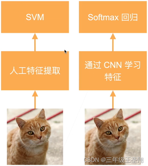
pointnet++代码逐行解析（一）——— train_classification

引起了计算机视觉方法论的改变，之前都是人工从图片提取特征，AlexNet使用CNN提取特征，如图3所示。

模型结构如下：

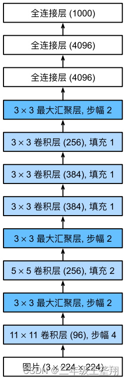
图中11×11卷积层（96）表示卷积核大小为11×11，输出通道数为96。

2.2 代码实现

AlexNet结构和LeNet类似，也使用nn.Sequential作为构造器。

import torch
from torch import nn
from d2l import torch as d2l

net = nn.Sequential(
    # 这里使用一个11*11的更大窗口来捕捉对象。
    # 同时，步幅为4，以减少输出的高度和宽度。
    # 另外，输出通道的数目远大于LeNet
    nn.Conv2d(1, 96, kernel_size=11, stride=4, padding=1), nn.ReLU(),
    nn.MaxPool2d(kernel_size=3, stride=2),
    # 减小卷积窗口，使用填充为2来使得输入与输出的高和宽一致，且增大输出通道数
    nn.Conv2d(96, 256, kernel_size=5, padding=2), nn.ReLU(),
    nn.MaxPool2d(kernel_size=3, stride=2),
    # 使用三个连续的卷积层和较小的卷积窗口。
    # 除了最后的卷积层，输出通道的数量进一步增加。
    # 在前两个卷积层之后，汇聚层不用于减少输入的高度和宽度
    nn.Conv2d(256, 384, kernel_size=3, padding=1), nn.ReLU(),
    nn.Conv2d(384, 384, kernel_size=3, padding=1), nn.ReLU(),
    nn.Conv2d(384, 256, kernel_size=3, padding=1), nn.ReLU(),
    nn.MaxPool2d(kernel_size=3, stride=2),
    nn.Flatten(),
    # 这里，全连接层的输出数量是LeNet中的好几倍。使用dropout层来减轻过拟合
    nn.Linear(6400, 4096), nn.ReLU(), nn.Dropout(p=0.5),
    nn.Linear(4096, 4096), nn.ReLU(), nn.Dropout(p=0.5),
    # 最后是输出层。由于这里使用Fashion-MNIST，所以用类别数为10，而非论文中的1000
    nn.Linear(4096, 10))

2.3 检查模型

检查模型即检查每层的名称及输出矩阵大小是否符合预期。

import torch
from torch import nn
from d2l import torch as d2l

net = nn.Sequential(
    # 这里使用一个11*11的更大窗口来捕捉对象。
    # 同时，步幅为4，以减少输出的高度和宽度。
    # 另外，输出通道的数目远大于LeNet
    nn.Conv2d(1, 96, kernel_size=11, stride=4, padding=1), nn.ReLU(),
    nn.MaxPool2d(kernel_size=3, stride=2),
    # 减小卷积窗口，使用填充为2来使得输入与输出的高和宽一致，且增大输出通道数
    nn.Conv2d(96, 256, kernel_size=5, padding=2), nn.ReLU(),
    nn.MaxPool2d(kernel_size=3, stride=2),
    # 使用三个连续的卷积层和较小的卷积窗口。
    # 除了最后的卷积层，输出通道的数量进一步增加。
    # 在前两个卷积层之后，汇聚层不用于减少输入的高度和宽度
    nn.Conv2d(256, 384, kernel_size=3, padding=1), nn.ReLU(),
    nn.Conv2d(384, 384, kernel_size=3, padding=1), nn.ReLU(),
    nn.Conv2d(384, 256, kernel_size=3, padding=1), nn.ReLU(),
    nn.MaxPool2d(kernel_size=3, stride=2),
    nn.Flatten(),
    # 这里，全连接层的输出数量是LeNet中的好几倍。使用dropout层来减轻过拟合
    nn.Linear(6400, 4096), nn.ReLU(), nn.Dropout(p=0.5),
    nn.Linear(4096, 4096), nn.ReLU(), nn.Dropout(p=0.5),
    # 最后是输出层。由于这里使用Fashion-MNIST，所以用类别数为10，而非论文中的1000
    nn.Linear(4096, 10))


X = torch.randn(1, 1, 224, 224)
for layer in net:
    X=layer(X)
    print(layer.__class__.__name__,'output shape:\t',X.shape)

# 输出如下：
Conv2d output shape: torch.Size([1, 96, 54, 54])
ReLU output shape: torch.Size([1, 96, 54, 54])
MaxPool2d output shape: torch.Size([1, 96, 26, 26])
Conv2d output shape: torch.Size([1, 256, 26, 26])
ReLU output shape: torch.Size([1, 256, 26, 26])
MaxPool2d output shape: torch.Size([1, 256, 12, 12])
Conv2d output shape: torch.Size([1, 384, 12, 12])
ReLU output shape: torch.Size([1, 384, 12, 12])
Conv2d output shape: torch.Size([1, 384, 12, 12])
ReLU output shape: torch.Size([1, 384, 12, 12])
Conv2d output shape: torch.Size([1, 256, 12, 12])
ReLU output shape: torch.Size([1, 256, 12, 12])
MaxPool2d output shape: torch.Size([1, 256, 5, 5])
Flatten output shape: torch.Size([1, 6400])
Linear output shape: torch.Size([1, 4096])
ReLU output shape: torch.Size([1, 4096])
Dropout output shape: torch.Size([1, 4096])
Linear output shape: torch.Size([1, 4096])
ReLU output shape: torch.Size([1, 4096])
Dropout output shape: torch.Size([1, 4096])
Linear output shape: torch.Size([1, 10])

2.4 训练模型

import torch
from torch import nn
from d2l import torch as d2l

net = nn.Sequential(
    # 这里使用一个11*11的更大窗口来捕捉对象。
    # 同时，步幅为4，以减少输出的高度和宽度。
    # 另外，输出通道的数目远大于LeNet
    nn.Conv2d(1, 96, kernel_size=11, stride=4, padding=1), nn.ReLU(),
    nn.MaxPool2d(kernel_size=3, stride=2),
    # 减小卷积窗口，使用填充为2来使得输入与输出的高和宽一致，且增大输出通道数
    nn.Conv2d(96, 256, kernel_size=5, padding=2), nn.ReLU(),
    nn.MaxPool2d(kernel_size=3, stride=2),
    # 使用三个连续的卷积层和较小的卷积窗口。
    # 除了最后的卷积层，输出通道的数量进一步增加。
    # 在前两个卷积层之后，汇聚层不用于减少输入的高度和宽度
    nn.Conv2d(256, 384, kernel_size=3, padding=1), nn.ReLU(),
    nn.Conv2d(384, 384, kernel_size=3, padding=1), nn.ReLU(),
    nn.Conv2d(384, 256, kernel_size=3, padding=1), nn.ReLU(),
    nn.MaxPool2d(kernel_size=3, stride=2),
    nn.Flatten(),
    # 这里，全连接层的输出数量是LeNet中的好几倍。使用dropout层来减轻过拟合
    nn.Linear(6400, 4096), nn.ReLU(), nn.Dropout(p=0.5),
    nn.Linear(4096, 4096), nn.ReLU(), nn.Dropout(p=0.5),
    # 最后是输出层。由于这里使用Fashion-MNIST，所以用类别数为10，而非论文中的1000
    nn.Linear(4096, 10))

batch_size = 128
train_iter, test_iter = d2l.load_data_fashion_mnist(batch_size, resize=224)
lr, num_epochs = 0.01, 10
d2l.train_ch6(net, train_iter, test_iter, num_epochs, lr, d2l.try_gpu())

# 输出如下：
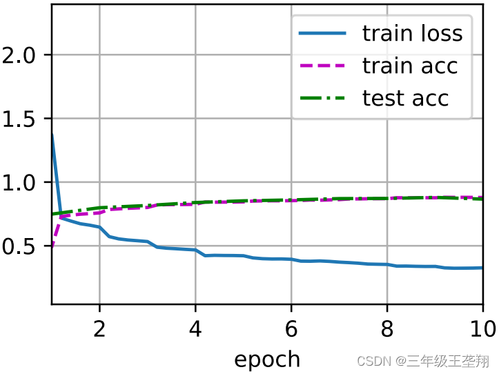
loss 0.327, train acc 0.879, test acc 0.866
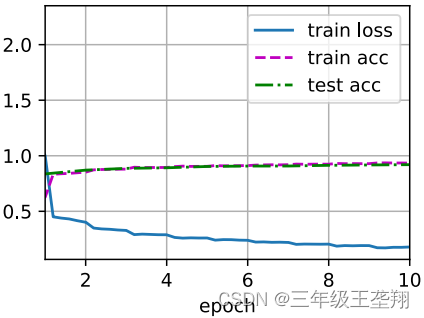
3903.6 examples/sec on cuda:0

训练过程如图5所示。

三、VGG

3.1 模型简介

VGG是在AlexNet上改进而来，可以看作是一个更大更深的AlexNet。

在同样计算开销下，深但窄的网络比浅但宽的网络好，因此VGG将AlexNet改造成更大更深的网络以提升性能。

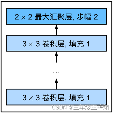
VGG是基于“块”的，VGG的“块”定义由多个卷积层和一个池化层组成，如图6所示。

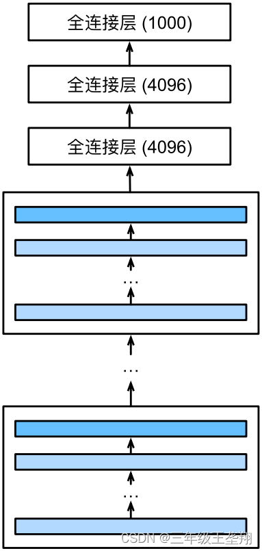
VGG的整体结构即由多个VGG“块”和几个全连接层组成，如图7所示。

3.2 代码实现

VGG块的实现

import torch
from torch import nn
from d2l import torch as d2l

def vgg_block(num_convs, in_channels, out_channels):
    layers = []
    for _ in range(num_convs):
        layers.append(nn.Conv2d(in_channels, out_channels, kernel_size=3, padding=1))
        layers.append(nn.ReLU())
        in_channels = out_channels
    layers.append(nn.MaxPool2d(kernel_size=2,stride=2))
    return nn.Sequential(*layers)

上述代码最后一行使用nn.Sequential(*layers)而不是nn.Sequential(layers)，是因为前者等价于将layers数组中所有内容取出放入Sequential，

例如：layers=[net1, net2, net3]

nn.Sequential(*layers)等价于nn.Sequential(net1, net2, net3)

而nn.Sequential(layers)等价于nn.Sequential([net1, net2, net3])

* 可以理解为C++中类似的意思，即取值。

每个“块”里使用的卷积核大小均为3×3，padding=1，stride默认为1，假设输入层大小为m×n，那么该层输出为(m+2)-3+1=m，(n+2)-3+1=n，故卷积层的输入输出大小相同。

池化层核尺寸为2×2，Stride=2，假设输入层大小为m×n，那么池化层输出为 $\frac{m-2}{2}+1=\frac{m}{2}$ ，n同理，因此每个VGG块的输出尺寸为输入的一半。

import torch
from torch import nn
from d2l import torch as d2l

def vgg_block(num_convs, in_channels, out_channels):
    layers = []
    for _ in range(num_convs):
        layers.append(nn.Conv2d(in_channels, out_channels, kernel_size=3, padding=1))
        layers.append(nn.ReLU())
        in_channels = out_channels
    layers.append(nn.MaxPool2d(kernel_size=2,stride=2))
    return nn.Sequential(*layers)

conv_arch = ((1, 64), (1, 128), (2, 256), (2, 512), (2, 512))

def vgg(conv_arch):
    conv_blks = []
    in_channels = 1
    # 卷积层部分
    for (num_convs, out_channels) in conv_arch:
        conv_blks.append(vgg_block(num_convs, in_channels, out_channels))
        in_channels = out_channels
    return nn.Sequential(
        *conv_blks, nn.Flatten(),
        # 全连接层部分
        nn.Linear(out_channels * 7 * 7, 4096), nn.ReLU(), nn.Dropout(0.5),
        nn.Linear(4096, 4096), nn.ReLU(), nn.Dropout(0.5),
        nn.Linear(4096, 10))
net = vgg(conv_arch)

3.3 检查模型

import torch
from torch import nn
from d2l import torch as d2l

def vgg_block(num_convs, in_channels, out_channels):
    layers = []
    for _ in range(num_convs):
        layers.append(nn.Conv2d(in_channels, out_channels, kernel_size=3, padding=1))
        layers.append(nn.ReLU())
        in_channels = out_channels
    layers.append(nn.MaxPool2d(kernel_size=2,stride=2))
    return nn.Sequential(*layers)

conv_arch = ((1, 64), (1, 128), (2, 256), (2, 512), (2, 512))

def vgg(conv_arch):
    conv_blks = []
    in_channels = 1
    # 卷积层部分
    for (num_convs, out_channels) in conv_arch:
        conv_blks.append(vgg_block(num_convs, in_channels, out_channels))
        in_channels = out_channels
    return nn.Sequential(
        *conv_blks, nn.Flatten(),
        # 全连接层部分
        nn.Linear(out_channels * 7 * 7, 4096), nn.ReLU(), nn.Dropout(0.5),
        nn.Linear(4096, 4096), nn.ReLU(), nn.Dropout(0.5),
        nn.Linear(4096, 10))
net = vgg(conv_arch)

X = torch.randn(size=(1, 1, 224, 224))
for blk in net:
    X = blk(X)
    print(blk.__class__.__name__,'output shape:\t',X.shape)

# 输出如下：
Sequential output shape: torch.Size([1, 64, 112, 112])
Sequential output shape: torch.Size([1, 128, 56, 56])
Sequential output shape: torch.Size([1, 256, 28, 28])
Sequential output shape: torch.Size([1, 512, 14, 14])
Sequential output shape: torch.Size([1, 512, 7, 7])
Flatten output shape: torch.Size([1, 25088])
Linear output shape: torch.Size([1, 4096])
ReLU output shape: torch.Size([1, 4096])
Dropout output shape: torch.Size([1, 4096])
Linear output shape: torch.Size([1, 4096])
ReLU output shape: torch.Size([1, 4096])
Dropout output shape: torch.Size([1, 4096])
Linear output shape: torch.Size([1, 10])

3.4 训练模型

import torch
from torch import nn
from d2l import torch as d2l

def vgg_block(num_convs, in_channels, out_channels):
    layers = []
    for _ in range(num_convs):
        layers.append(nn.Conv2d(in_channels, out_channels, kernel_size=3, padding=1))
        layers.append(nn.ReLU())
        in_channels = out_channels
    layers.append(nn.MaxPool2d(kernel_size=2,stride=2))
    return nn.Sequential(*layers)

conv_arch = ((1, 64), (1, 128), (2, 256), (2, 512), (2, 512))

def vgg(conv_arch):
    conv_blks = []
    in_channels = 1
    # 卷积层部分
    for (num_convs, out_channels) in conv_arch:
        conv_blks.append(vgg_block(num_convs, in_channels, out_channels))
        in_channels = out_channels
    return nn.Sequential(
        *conv_blks, nn.Flatten(),
        # 全连接层部分
        nn.Linear(out_channels * 7 * 7, 4096), nn.ReLU(), nn.Dropout(0.5),
        nn.Linear(4096, 4096), nn.ReLU(), nn.Dropout(0.5),
        nn.Linear(4096, 10))
net = vgg(conv_arch)

ratio = 4
small_conv_arch = [(pair[0], pair[1] // ratio) for pair in conv_arch]
net = vgg(small_conv_arch)

lr, num_epochs, batch_size = 0.05, 10, 128
train_iter, test_iter = d2l.load_data_fashion_mnist(batch_size, resize=224)
d2l.train_ch6(net, train_iter, test_iter, num_epochs, lr, d2l.try_gpu())

# 输出如下
loss 0.179, train acc 0.934, test acc 0.920
2390.1 examples/sec on cuda:0

训练过程如图8所示。

四、NiN（网络中的网络）

NiN（NetWork in NetWork）是为了解决全连接层参数过多，容易造成过拟合的问题而提出。思想类似SharedMLP。使用大小为1×1的卷积核整合信息。

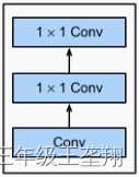
NiN的基本单元为NiN块，一个NiN块由一个普通卷积层和2个SharedMLP组成，如图9所示。

NiN网络参数少，不容易过拟合。

NiN网络结构如下：

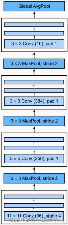
最后一层Global AvgPool表示池化过程中的核长宽和输入一致，对应pytorch中的函数为nn.AdaptiveAvgPool2d((1, 1))。

代码实现及训练和前述三个模型类似，不再赘述。

五、GoogLeNet（含并行连接的网络）

设计GoogLeNet的动机是前面的网络通过不同的结构设计，起到了不同的效果，如今我有几个备选的网络结构，那么选择哪个能取到较好的效果？

这个问题的答案很难得知，但是每种网络结构肯定都能提取某方面特征，既然这样，我就把所有备选的网络结构都用上去，那么就能获取这几种结构网络所能提取的所有类型的特征。

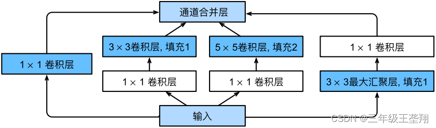
GoogLeNet 的核心部分为 Inception 块，其结果如图11所示。注意看几个分支可知每个分支都不改变输入数据的长宽，只改变通道数，几个分支的输出在通道上叠加，例如四个分支的输出通道数均为2，合并后数据的通道数为8，因此 Inception 块不改变输入数据的高宽，只改变通道数。

使用Inception块可以降低参数量及计算复杂度，如图12所示，图12(a)中输入输出通道数分别为192、256，使用不同的网络实现相同的通道数输出所对应的参数量和计算复杂度如图12(b)所示，可见使用 Inception 块可以降低参数量及计算复杂度。

（a）Inception 块各部分通道数（b）参数量和计算复杂度对比
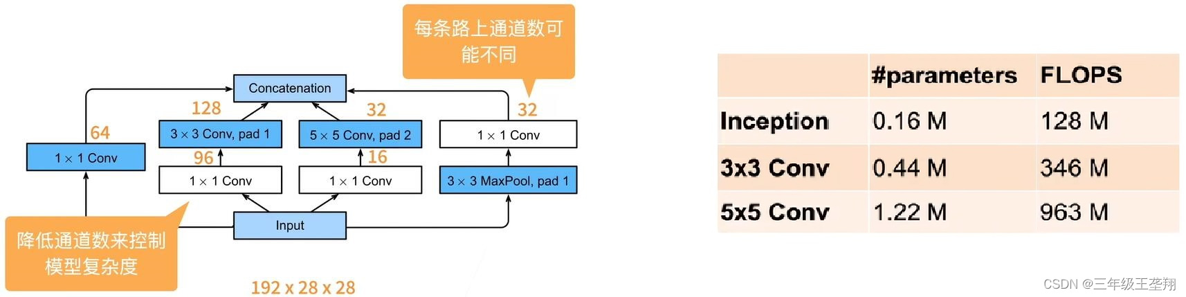
**图12.** Inception 块通道数与对应的参数、计算复杂度

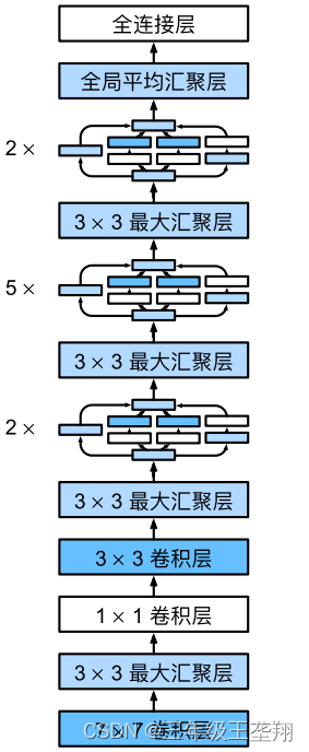
GoogLeNet 的结构如图13所示，图中汇聚层即池化层，可见使用了很多 Inception 块。

六、ResNet

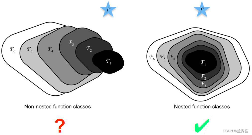
残差网络的核心思想如图14所示，图中 $f^{*}$ 是最优解，区域从 $\mathcal{F}_1$ 到 $\mathcal{F}_6$ 表示对着网络层数的加深，整个模型所能表达的函数范围，即层数越深表达的函数越多。

然而从左图看，随着层数的增多，从 $\mathcal{F}_1$ 到 $\mathcal{F}_6$ ，区域并没有越来越接近 $f^{*}$

从右图看，从 $\mathcal{F}_1$ 到 $\mathcal{F}_6$ ，区域是逐渐更加接近 $f^{*}$ 的，说明在这种情况下加深层数，有利于获得更好的结果。

因此从图14可知，如果通过加深层数，可以使增加层数后的模型完全包含之前的模型，就可以通过增加层数获得更好的模型。

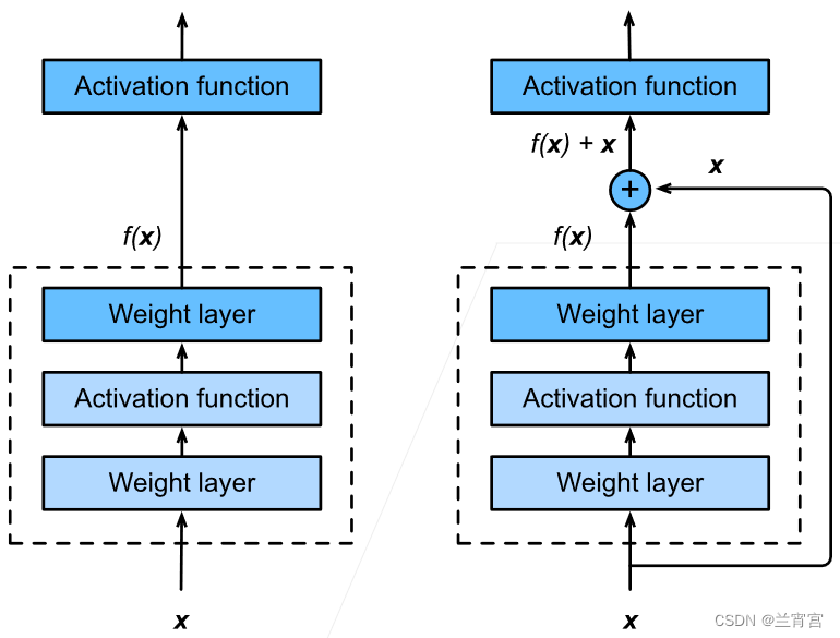
做法也很简单，构建 $f\left ( x \right )=x+g\left ( x \right )$ 的结构，其中 $x$ 表示原始的层， $g\left ( x \right )$ 表示新加的层，这样即使 $g\left ( x \right )$ 什么都不做， $f\left ( x \right )$ 至少可以表达 $x$ 。例如 $g\left ( x \right )=ax^2+b\sin\left ( x \right )$ ，那么显然带参数的函数 $f\left ( x \right )=x+g\left ( x \right )=x+ax^2+b\sin\left ( x \right )$ 在 $\left\{\begin{matrix} a=0\\ b=0 \end{matrix}\right.$ 时可以表达 $f\left ( x \right )=x$ 。

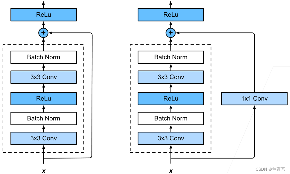
实现过程如图15所示，在激活函数前通过右边的快速通道将上一层的输出结果加上来。

当直接加加不上去的话可以通过在快速通道上增加一个简单层进行变换，如图16所示。

总结：

残差块使得很深的网络更加容易训练。甚至可以训练一千层的网络

残差网络对随后的深层神经网络设计产生了深远影响，无论是卷积类网络还是全连接类网络。

代码实现：

import torch
from torch import nn
from torch.nn import functional as F
from d2l import torch as d2l

class Residual(nn.Module):  
    def __init__(self, input_channels, num_channels, use_1x1conv=False,
                 strides=1):
        super().__init__()
        self.conv1 = nn.Conv2d(input_channels, num_channels, kernel_size=3,
                               padding=1, stride=strides)
        self.conv2 = nn.Conv2d(num_channels, num_channels, kernel_size=3,
                               padding=1)
        if use_1x1conv:
            self.conv3 = nn.Conv2d(input_channels, num_channels,
                                   kernel_size=1, stride=strides)
        else:
            self.conv3 = None # 快速通道上的变换层
        self.bn1 = nn.BatchNorm2d(num_channels)
        self.bn2 = nn.BatchNorm2d(num_channels)
        self.relu = nn.ReLU(inplace=True)

    def forward(self, X):
        Y = F.relu(self.bn1(self.conv1(X)))
        Y = self.bn2(self.conv2(Y))
        if self.conv3:
            X = self.conv3(x)
        Y += X
        return F.relu(Y)