机器学习入门（1）：导论Introduction、线性回归Liner Regression-优快云博客

本文链接：https://blog.youkuaiyun.com/qq_20537963/article/details/129903718

文章介绍了吴恩达的机器学习课程，涵盖了监督学习，包括回归和分类，无监督学习，如聚类算法和降维，以及强化学习的基本概念。同时，讨论了线性回归模型的误差和成本函数，并详细阐述了梯度下降法在优化参数中的应用。

摘要生成于 C知道，由 DeepSeek-R1 满血版支持，前往体验 >

吴恩达机器学习视频链接第一周

Week1

导入

机器学习包括：

监督学习 Supervised Learning
无监督学习 Unsupervised Learning
强化学习 Reinforce Learning

监督学习

训练：给数据集x和标签y
期待：仅仅给出x，预测出y

监督学习分类：

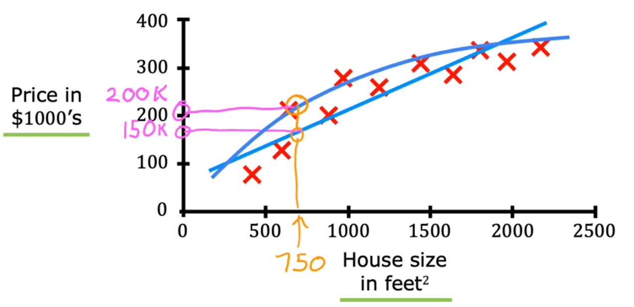
回归

Predict a number from infinitely many possible outputs

在这里插入图片描述

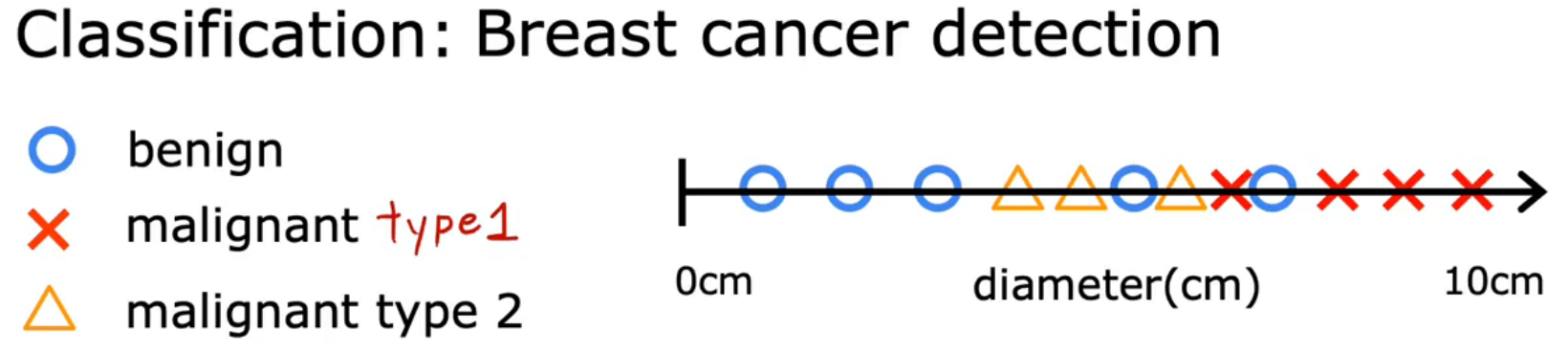
分类

Trying to predict only a small limitied number of classifies or categories——disperse

The case of One input:

在这里插入图片描述
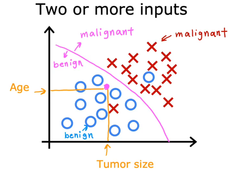
Multiple inputs:

无监督学习

有输入x，没有标签y

在这里插入图片描述

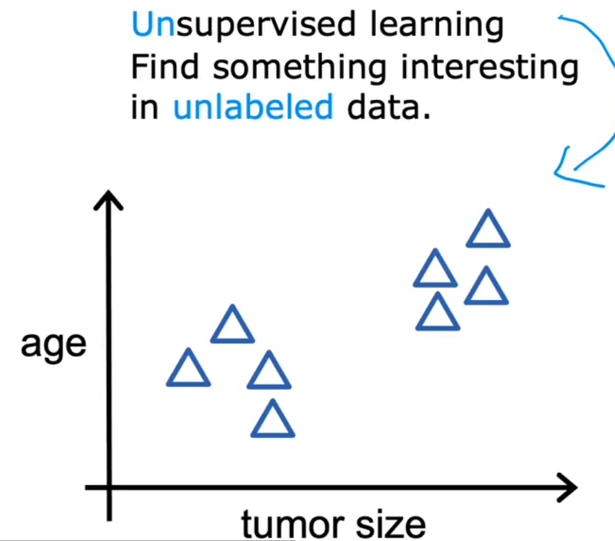
无监督学习分类：

聚类算法Clustering

将未标记的数据放到不同的簇中

examlpes:

谷歌新闻
DNA序列
市场细分

异常检测Anomaly detection

降维Dimensionality reduction

3.回归模型

术语 Terminology

Training set
$x$ = input variable / feature
$y$ = output / target variable
$m$ = total number of training examples
$(x, y)$ = single training example
$x^{(i)},y^{(i)})$ = the $i^{th}$ training example
- i == a specific column
$\widehat{y}$ (y hat): prediction or estimate

在这里插入图片描述

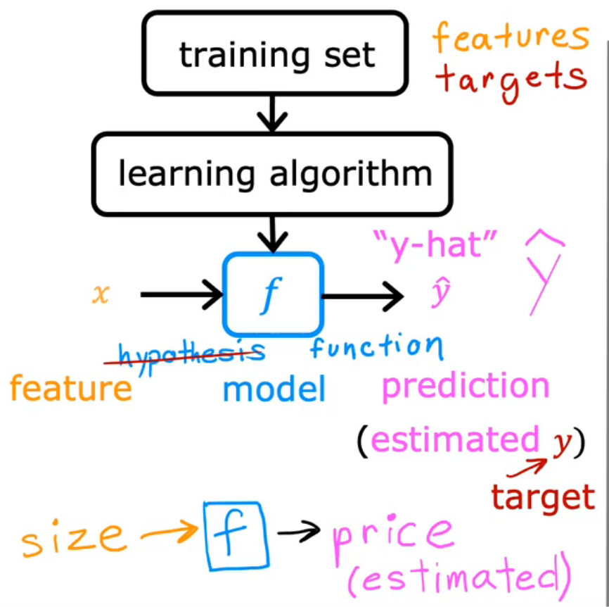
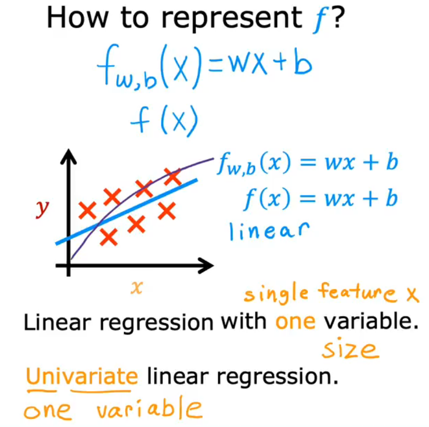
how to express f？—Liner regression

say the f is a linear function

在这里插入图片描述

Cost function

$f (x) = w x + b$

w,b:parameters
- w:coefficients
- b:weights

在这里插入图片描述

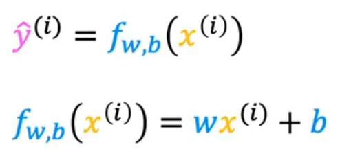
Cost Function

review: $f_{w,b}(x^{(i)})=wx^{(i)}+b$

error : $\widehat{y}^{(i)}-y^{(i)}$
Cost function(Squared error cost function 方差代价函数):
- $J(w,b)=\frac1{2m}\sum_{i=1}^{m}(\widehat{y}^{(i)}-y^{(i)})^2$
as we substitute the $\widehat{y}$ with $f_{w,b}x^{(i)}$ , it changes to:
- $J(w,b)=\frac1{2m}\sum_{i=1}^m(f_{w,b}x^{(i)}-y^{(i)})^2$

Cost function Intution—the relation between f(w) and J(w)

in the first part, we ignore $b$
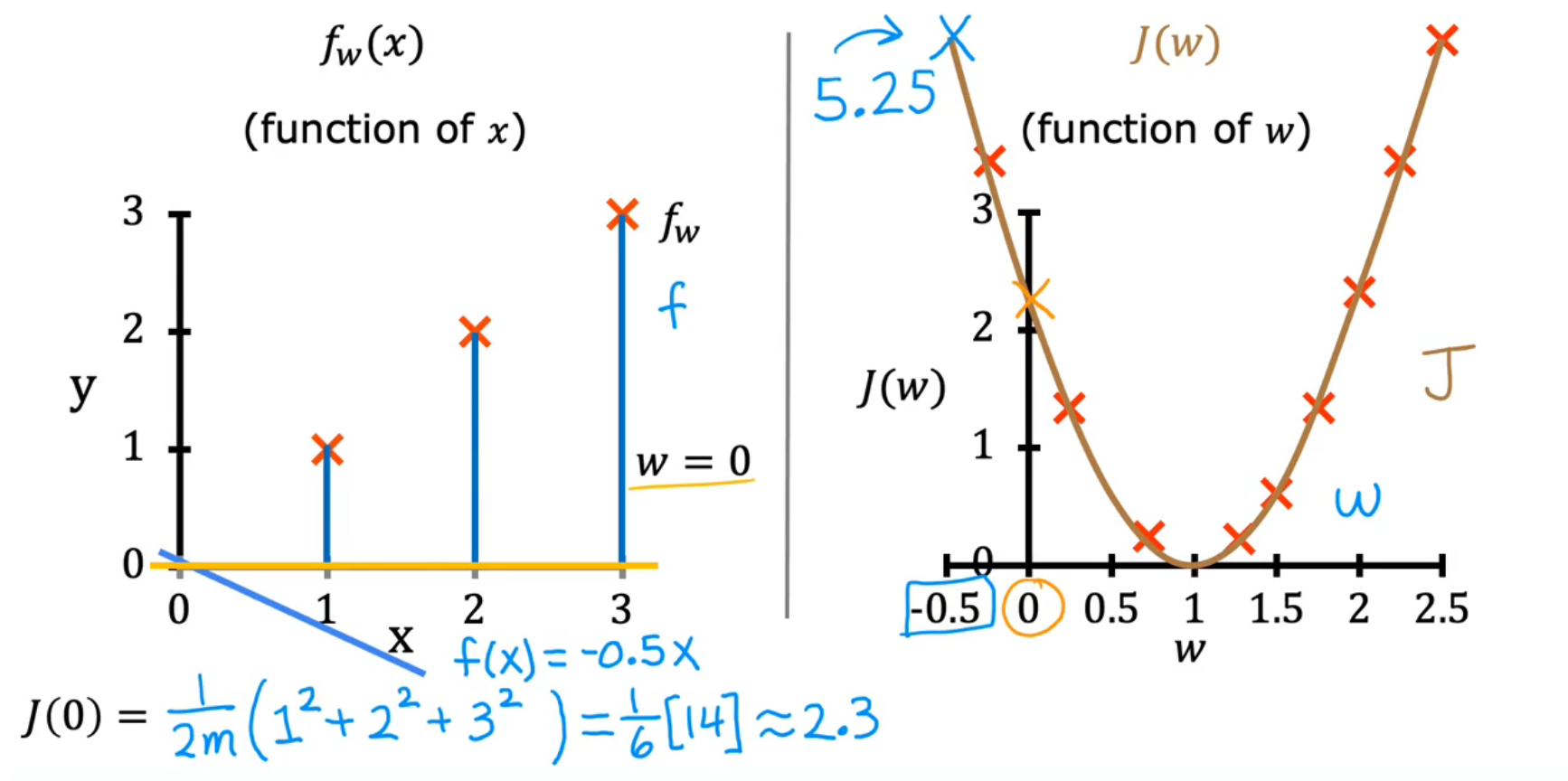
the second part:

在这里插入图片描述

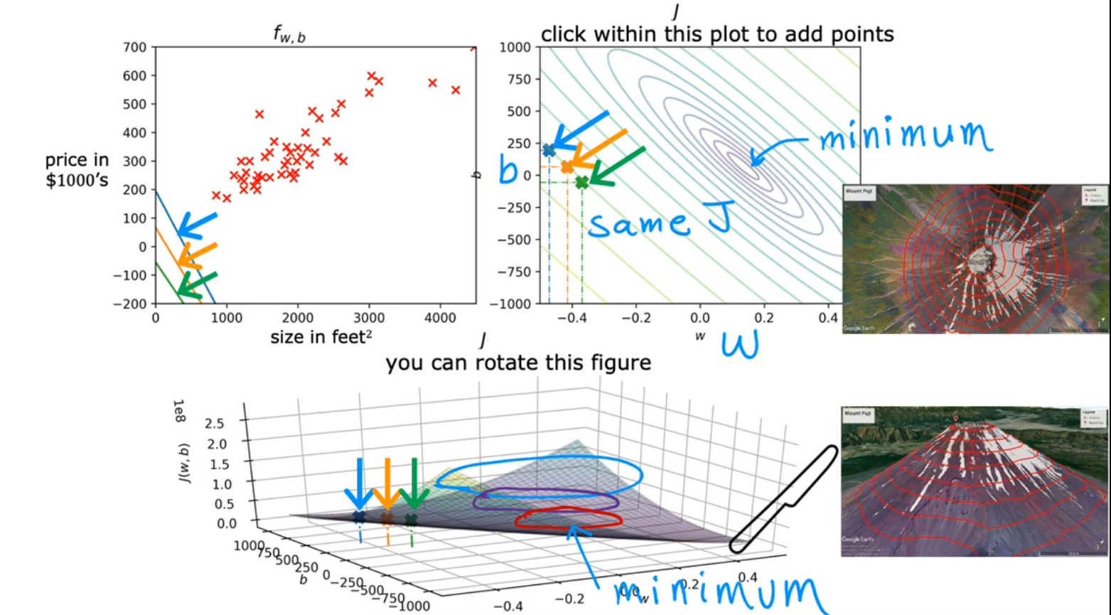
To approach the lowest point

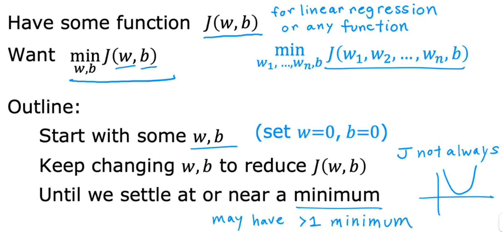
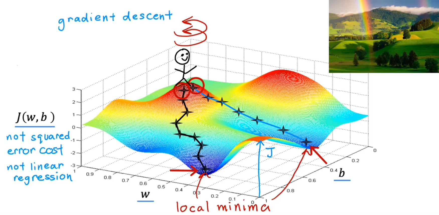
4. Gradient decent梯度下降法

Problem description

在这里插入图片描述

The Visuable model:

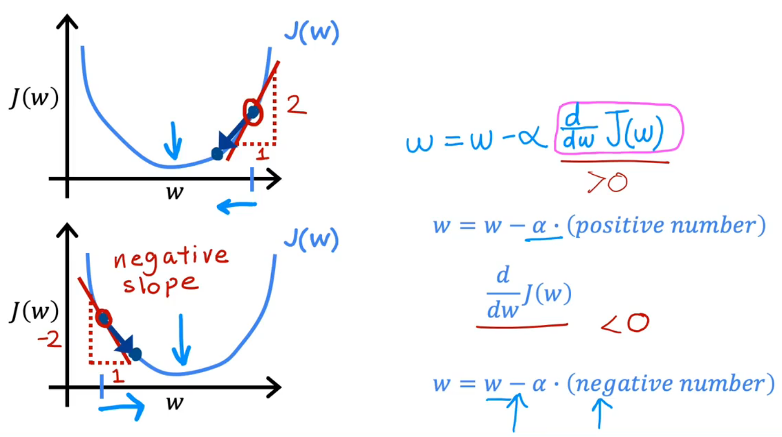
Gradient decent algorithm

$w=w-\alpha\frac\partial{\partial w}J(w,b)$
$\alpha$ means Learning rate

Algorithm description

The right way of updating w and b is ----- Simultaneous update

Ordered Steps:

$tmp\_w=w-\alpha\frac\partial{\partial w}J(w,b)$
$tmp\_b=b-\alpha\frac{\partial}{\partial b}J(w,b)$
$w=tmp\_w$
$b=tmp\_b$

which $\partial$ means partial derivative

Intution understangding of gradient descent

在这里插入图片描述

Learning Rate

Too small: It will take a long time by each going a tiny tiny baby step
Too large:
- Overshoot, never reach minimum
- Or, Fail to converge, even diverge