图像处理工具- scikit-image

scikit-image图像数据处理

Color 模块和exposure模块

1.基本操作

import numpy as np
import matplotlib.pyplot as plt
from skimage import data

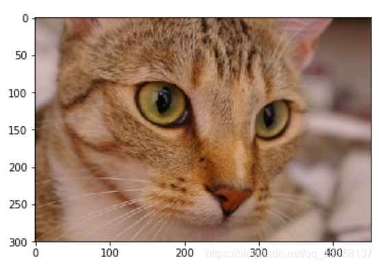
color_image = data.chelsea()
print(color_image.shape)
plt.imshow(color_image)
answer：
(300, 451, 3)

2.分割和索引

red_channel = color_image[:, :, 0]  # 红色通道
plt.imshow(red_channel, cmap='gray')
print(red_channel.shape)
answer：
(300, 451)

色彩空间 RGB,HSV,Gray

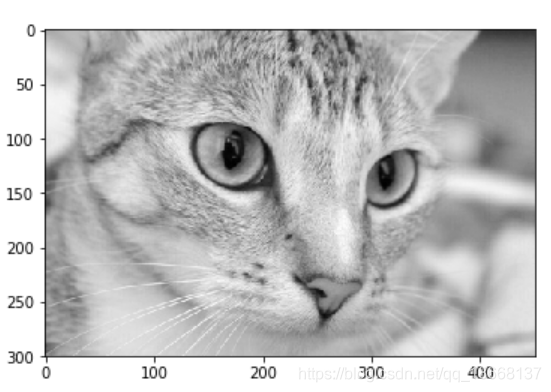
• RGB转gray  -- skimage.color.rgb2gray()

  import skimage
  
  gray_img = skimage.color.rgb2gray(color_image)
  plt.imshow(gray_img, cmap='gray')
  print(gray_img.shape)
  answer:
  (300,451)

   

颜色直方图

• 能快速描绘图像整体像素值分布的统计信息
  • skimage.exposure.histogram
  • 可以根据直方图选定阈值用于调节图像对比度
• 对比度：
  • 增强图像数据的对比度有利于特征的提取，不论是从肉眼还是算法来看都有帮助
  • 更改对比度范围
    • skimage.exposure.rescale_intensity(image,in_range=(min,max))，原图中小于min的像素值设为0，大鱼max的为255
  • 直方图均衡化
    • 自动调整图像对比度 skimage.exposure.equalize_hist(image),处理好数据范围变为【0，1】

• from skimage import data
  from skimage import exposure
  
  # 灰度图颜色直方图
  image = data.camera()
  #print(image.shape)
  
  hist, bin_centers = exposure.histogram(image) #bin_centers是像素值的范围，这里输出是0-255
  print(bin_centers)
  fig, ax = plt.subplots(ncols=1)
  ax.fill_between(bin_centers, hist)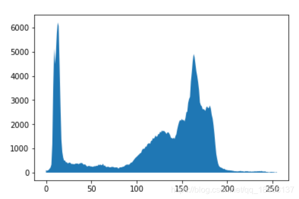

  

• 彩色图像直方图

• # 彩色图像直方图
  cat = data.chelsea()
  
  # R通道
  hist_r, bin_centers_r = exposure.histogram(cat[:,:,0])
  # G通道
  hist_g, bin_centers_g = exposure.histogram(cat[:,:,1])
  # B通道
  hist_b, bin_centers_b = exposure.histogram(cat[:,:,2])
  
  fig, (ax_r, ax_g, ax_b) = plt.subplots(ncols=3, figsize=(10, 5))
  #ax = plt.gca()
  ax_r.fill_between(bin_centers_r, hist_r)
  ax_g.fill_between(bin_centers_g, hist_g)
  ax_b.fill_between(bin_centers_b, hist_b)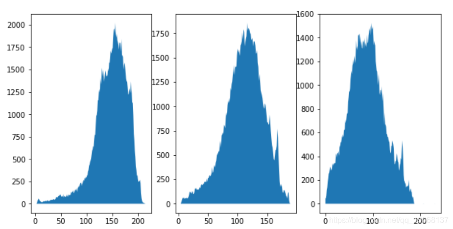

  

对比度

# 原图像
image = data.camera()
hist, bin_centers = exposure.histogram(image)

# 改变对比度
# image中小于10的像素值设为0，大于180的像素值设为255
high_contrast = exposure.rescale_intensity(image, in_range=(10, 180))
hist2, bin_centers2 = exposure.histogram(high_contrast)

# 图像对比 
fig, (ax_1, ax_2) = plt.subplots(ncols=2, figsize=(10, 5))
ax_1.imshow(image, cmap='gray')
ax_2.imshow(high_contrast, cmap='gray')

fig, (ax_hist1, ax_hist2) = plt.subplots(ncols=2, figsize=(10, 5))
ax_hist1.fill_between(bin_centers, hist)
ax_hist2.fill_between(bin_centers2, hist2)

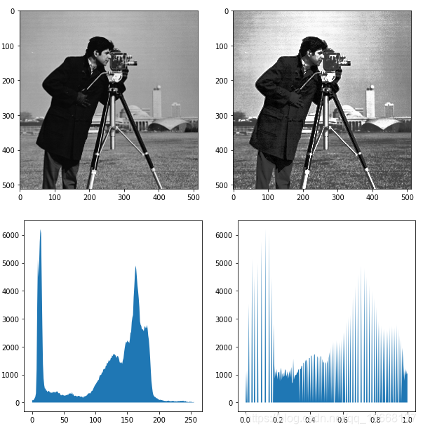
自动直方图均衡化

# 直方图均衡化
equalized = exposure.equalize_hist(image)
hist3, bin_centers3 = exposure.histogram(equalized)

# 图像对比 
fig, (ax_1, ax_2) = plt.subplots(ncols=2, figsize=(10, 5))
ax_1.imshow(image, cmap='gray')
ax_2.imshow(equalized, cmap='gray')

fig, (ax_hist1, ax_hist2) = plt.subplots(ncols=2, figsize=(10, 5))
ax_hist1.fill_between(bin_centers, hist)
ax_hist2.fill_between(bin_centers3, hist3)

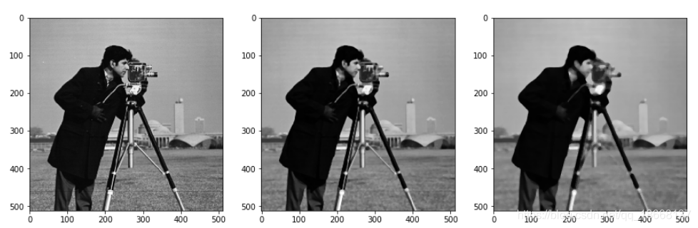
图像滤波

• 滤波可以去除图像中的噪声点，由此增强图像的特征
• 中值滤波
  • skimage.filters.rank.median

from skimage import data
from skimage.morphology import disk
from skimage.filters.rank import median

img = data.camera()
med1 = median(img, disk(3)) # 3x3中值滤波
med2 = median(img, disk(5)) # 5x5中值滤波

# 图像对比 
fig, (ax_1, ax_2, ax_3) = plt.subplots(ncols=3, figsize=(15, 10))
ax_1.imshow(img, cmap='gray')
ax_2.imshow(med1, cmap='gray')
ax_3.imshow(med2, cmap='gray')

 

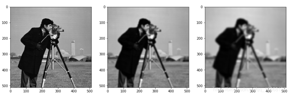
• 高斯滤波
  • skimage.filters.gaussian

from skimage import data
from skimage.morphology import disk
from skimage.filters import gaussian

img = data.camera()
gas1 = gaussian(img, sigma=3) # sigma=3
gas2 = gaussian(img, sigma=5) # sigma=5

# 图像对比 
fig, (ax_1, ax_2, ax_3) = plt.subplots(ncols=3, figsize=(15, 10))
ax_1.imshow(img, cmap='gray')
ax_2.imshow(gas1, cmap='gray')
ax_3.imshow(gas2, cmap='gray')