rEDM的用法（4）——Tracking interaction strength using S-map

Load package and time series

In this demonstration, we use the same time series generated from the 5-species model (Resource, Consumer1, Consumer2, Predator1, Predator2) following Deyle et al. (2016).

## Load package and data
library(rEDM) 
d <- read.csv("ESM5_Data_5spModel.csv")

Set parameters and do S-map

In this demonstration, we focus on the effects on Consumer1 (C1). As shown in Deyle et al. (2016), the effects of Predator2 (P2) on C1 are negligible, and thus we ignore P2 in the embedding. We use fully multivariate embedding (Deyle et al. 2016, Deyle et al. 2011) in order to investigate effects of R, C2, and P1 on C1.

# Make multivariate embedding
Embedding <- c("R","C1","C2","P1")
block <- d[,Embedding]
# Normalize data
block <- as.data.frame(apply(block, 2, function(x) (x-mean(x))/sd(x)))

# Define the target column (C1 = column 2)
targ_col <- 2

# Please reduce the number of data points if the calculation takes long
data_used <- 1:2000

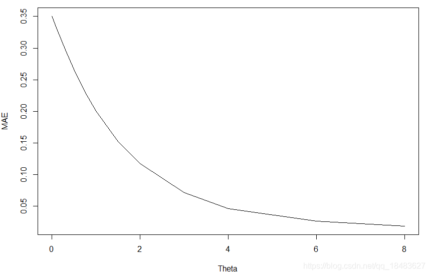
# Explore the best weighting parameter (nonlinear parameter = theta)
# Best theta is selected based on mean absolute error (MAE)
test_theta <- block_lnlp(block[data_used,],
                         method = "s-map",
                         num_neighbors = 0, # We have to use any value < 1 for s-map
                         theta = c(0, 1e-04, 3e-04, 0.001,
                                   0.003, 0.01, 0.03, 0.1,
                                   0.3, 0.5, 0.75, 1, 1.5,
                                   2, 3, 4, 6, 8), # We try many thetas to find the best parameter
                         target_column = targ_col, # Specify the target column
                         silent = T)

# Check MAE and theta
plot(test_theta$mae~test_theta$theta, type="l", xlab="Theta", ylab="MAE")

# Best theta = 8 in this case
best_theta <- test_theta[which.min(test_theta$mae),"theta"]

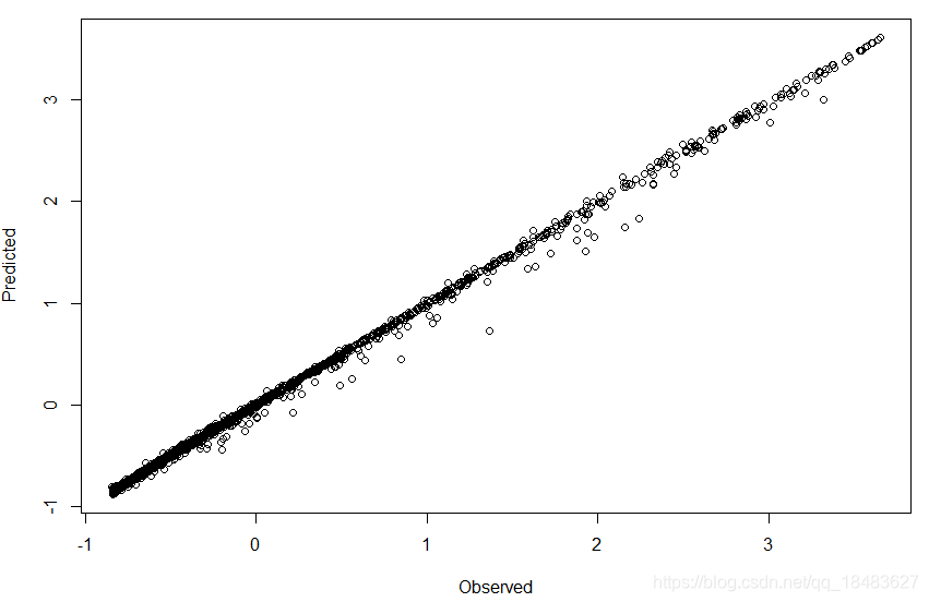
# Do S-map analysis with the best theta
smap_res <-  block_lnlp(block[data_used,],
                        method = "s-map",
                        num_neighbors = 0, # we have to use any value < 1 for s-map
                        theta = best_theta,
                        target_column = targ_col,
                        silent = T,
                        save_smap_coefficients = T) # save S-map coefficients

#### Visualize results
## Observed v.s. Predicted
smap_out <- as.data.frame(smap_res$model_output[[1]])
plot(smap_out$obs, smap_out$pred, xlab="Observed", ylab="Predicted")
## Time series of fluctuating interaction strength
smap_coef <- as.data.frame(smap_res$smap_coefficients[[1]])
colnames(smap_coef) <- c("dC1dR","dC1dC1","dC1dC2","dC1dP1","Intercept")

# Plot all partial derivatives
trange <- 1:200
windows(width=6, height=4)
plot(smap_coef[trange,"dC1dR"],
     type="l", col="royalblue", lwd=2, xlab="time",
     ylab="Interction strength", ylim = c(-1.0, 2.5),
     main = "Fluctuating interaction strength")
lines(smap_coef[trange,"dC1dC2"], lwd=2, col="red3")
lines(smap_coef[trange,"dC1dP1"], lwd=2, col="springgreen3")
abline(a=0 ,b=0 , lty="dashed", col="black", lwd=.5)

修改了原代码中的一些小错误。

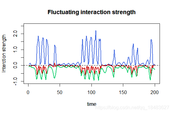
As can be seen in Figure 7 in the main text, interaction strengths fluctuate with time.

References

Deyle E, Sugihara G (2011) Generalized theorems for nonlinear state space reconstruction. PLoS ONE 6: e18295.(PDF)

Deyle ER, May RM, Munch SB, Sugihara G (2016) Tracking and forecasting ecosystem interactions in real time. Proc R Soc Lond B Biol Sci 283: 20152258.(PDF)