


 本文通过Python和SQL对京东用户行为数据进行分析,包括流量指标、消费频次、时间分布、转化漏斗和留存率。数据显示,网站购物体验良好,但跳失率较高,复购率和转化率有待提升。建议优化搜索功能,提供一键购物,加强用户召回和互动,提高用户粘性和留存率。
1、项目背景
项目对京东电商运营数据集进行指标分析以了解用户购物行为特征,为运营决策提供支持建议。本文采用了MySQL和Python两种代码进行指标计算以适应不同的数据分析开发环境。
2、数据集介绍
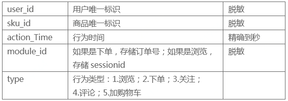
数据集共有五个文件,包含了'2018-02-01'至'2018-04-15'之间的用户数据,数据已进行了脱敏处理,本文使用了其中的行为数据表,表中共有五个字段,各字段含义如下图所示:
3、数据清洗
# 导入python相关模块
import numpy as np
import pandas as pd
import seaborn as sns
import matplotlib.pyplot as plt
from datetime import datetime
plt.style.use('ggplot')

%matplotlib inline

# 设置中文编码和负号的正常显示
plt.rcParams['font.sans-serif']=['SimHei']
plt.rcParams['axes.unicode_minus']=False
# 读取数据,数据集较大,如果计算机读取内存不够用,可以尝试kaggle比赛
# 中的reduce_mem_usage函数,附在文末,主要原理是把int64/float64
# 类型的数值用更小的int(float)32/16/8来搞定
user_action = pd.read_csv('jdata_action.csv')
# 因数据集过大,本文截取'2018-03-30'至'2018-04-15'之间的数据完成本次分析
# 注:仅4月份的数据包含加购物车行为,即type == 5
user_data = user_action[(user_action['action_time'] > '2018-03-30') & (user_action['action_time'] < '2018-04-15')]
# 存至本地备用
user_data.to_csv('user_data.csv',sep=',')
# 查看原始数据各字段类型
behavior = pd.read_csv('user_data.csv', index_col=0)
behavior[:10]
output
user_id sku_id action_time module_id type 17 1455298 208441 2018-04-11 15:21:43 6190659 1 18 1455298 334318 2018-04-11 15:14:54 6190659 1 19 1455298 237755 2018-04-11 15:14:13 6190659 1 20 1455298 6422 2018-04-11 15:22:25 6190659 1 21 1455298 268566 2018-04-11 15:14:26 6190659 1 22 1455298 115915 2018-04-11 15:13:35 6190659 1 23 1455298 208254 2018-04-11 15:22:16 6190659 1 24 1455298 177209 2018-04-14 14:09:59 6628254 1 25 1455298 71793 2018-04-14 14:10:29 6628254 1 26 1455298 141950 2018-04-12 15:37:53 10207258 1behavior.info()
output
<class 'pandas.core.frame.DataFrame'>
Int64Index: 7540394 entries, 17 to 37214234
Data columns (total 5 columns):
user_id int64
sku_id int64
action_time object
module_id int64
type           int64
dtypes: int64(4), object(1)
memory usage: 345.2+ MB
# 查看缺失值
behavior.isnull().sum()
output
user_id 0
sku_id 0
action_time 0
module_id 0
type           0
dtype: int64
数据各列无缺失值。
# 原始数据中时间列action_time,时间和日期是在一起的,不方便分析,对action_time列进行处理,拆分出日期和时间列,并添加星期字段求出每天对应
# 的星期,方便后续按时间纬度对数据进行分析
behavior['date'] = pd.to_datetime(behavior['action_time']).dt.date # 日期
behavior['hour'] = pd.to_datetime(behavior['action_time']).dt.hour # 时间
behavior['weekday'] = pd.to_datetime(behavior['action_time']).dt.weekday_name # 周
# 去除与分析无关的列
behavior = behavior.drop('module_id', axis=1)
# 将用户行为标签由数字类型改为用字符表示
behavior_type = {1:'pv',2:'pay',3:'fav',4:'comm',5:'cart'}
behavior['type'] = behavior['type'].apply(lambda x: behavior_type[x])
behavior.reset_index(drop=True,inplace=True)
# 查看处理好的数据
behavior[:10]
output
user_id   sku_id   action_time   type   date   hour   weekday
0   1455298   208441   2018-04-11 15:21:43   pv   2018-04-11   15   Wednesday
1   1455298   334318   2018-04-11 15:14:54   pv   2018-04-11   15   Wednesday
2   1455298   237755   2018-04-11 15:14:13   pv   2018-04-11   15   Wednesday
3   1455298   6422   2018-04-11 15:22:25   pv   2018-04-11   15   Wednesday
4   1455298   268566   2018-04-11 15:14:26   pv   2018-04-11   15   Wednesday
5   1455298   115915   2018-04-11 15:13:35   pv   2018-04-11   15   Wednesday
6   1455298   208254   2018-04-11 15:22:16   pv   2018-04-11   15   Wednesday
7   1455298   177209   2018-04-14 14:09:59   pv   2018-04-14   14   Saturday
8   1455298   71793   2018-04-14 14:10:29   pv   2018-04-14   14   Saturday
9   1455298   141950   2018-04-12 15:37:53   pv   2018-04-12   15   Thursday
4、分析模型构建指标
1.流量指标分析
pv、uv、消费用户数占比、消费用户总访问量占比、消费用户人均访问量、跳失率。
PV UV
# 总访问量
pv = behavior[behavior['type'] == 'pv']['user_id'].count()
# 总访客数
uv = behavior['user_id'].nunique()
# 消费用户数
user_pay = behavior[behavior['type'] == 'pay']['user_id'].unique()
# 日均访问量
pv_per_day = pv / behavior['date'].nunique()
# 人均访问量
pv_per_user = pv / uv
# 消费用户访问量
pv_pay = behavior[behavior['user_id'].isin(user_pay)]['type'].value_counts().pv
# 消费用户数占比
user_pay_rate = len(user_pay) / uv
# 消费用户访问量占比
pv_pay_rate = pv_pay / pv
# 消费用户人均访问量
pv_per_buy_user = pv_pay / len(user_pay)
# SQL
SELECT count(DISTINCT user_id) UV,
(SELECT count(*) PV from behavior_sql WHERE type = 'pv') PV
FROM behavior_sql;

SELECT count(DISTINCT user_id)
FROM behavior_sql
WHERE WHERE type = 'pay';

SELECT type, COUNT(*) FROM behavior_sql
WHERE
user_id IN
(SELECT DISTINCT user_id
FROM behavior_sql
WHERE type = 'pay')
AND type = 'pv'
GROUP BY type;
print('总访问量为 %i' %pv)
print('总访客数为 %i' %uv)
print('消费用户数为 %i' %len(user_pay))
print('消费用户访问量为 %i' %pv_pay)
print('日均访问量为 %.3f' %pv_per_day)
print('人均访问量为 %.3f' %pv_per_user)
print('消费用户人均访问量为 %.3f' %pv_per_buy_user)
print('消费用户数占比为 %.3f%%' %(user_pay_rate * 100))
print('消费用户访问量占比为 %.3f%%' %(pv_pay_rate * 100))
output
总访问量为 6229177
总访客数为 728959
消费用户数为 395874
消费用户访问量为 3918000
日均访问量为 389323.562
人均访问量为 8.545
消费用户人均访问量为 9.897
消费用户数占比为 54.307%
消费用户访问量占比为 62.898%
消费用户人均访问量和总访问量占比都在平均值以上,有过消费记录的用户更愿意在网站上花费更多时间,说明网站的购物体验尚可,老用户对网站有一定依赖性,对没有过消费记录的用户要让快速了解产品的使用方法和价值,加强用户和平台的黏连。
跳失率
# 跳失率:只进行了一次操作就离开的用户数/总用户数
attrition_rates = sum(behavior.groupby('user_id')['type'].count() == 1) / (behavior['user_id'].nunique())
# SQL
SELECT
(SELECT COUNT(*)
FROM (SELECT user_id
FROM behavior_sql GROUP BY user_id
HAVING COUNT(type)=1) A) /
(SELECT COUNT(DISTINCT user_id) UV FROM behavior_sql) attrition_rates;
print('跳失率为 %.3f%%' %(attrition_rates * 100) )
output
跳失率为 22.585%
整个计算周期内跳失率为22.585%,还是有较多的用户仅做了单次操作就离开了页面,需要从首页页面布局以及产品用户体验等方面加以改善,提高产品吸引力。
2、用户消费频次分析
# 单个用户消费总次数
total_buy_count = (behavior[behavior['type']=='pay'].groupby(['user_id'])['type'].count()
.to_frame().rename(columns={'type':'total'}))
# 消费次数前10客户
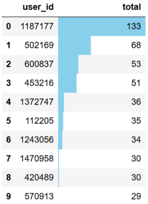
topbuyer10 = total_buy_count.sort_values(by='total',ascending=False)[:10]
# 复购率
re_buy_rate = total_buy_count[total_buy_count>=2].count()/total_buy_count.count()
# SQL
#消费次数前10客户
SELECT user_id, COUNT(type) total_buy_count
FROM behavior_sql
WHERE type = 'pay'
GROUP BY user_id
ORDER BY COUNT(type) DESC
LIMIT 10

#复购率
CREAT VIEW v_buy_count
AS SELECT user_id, COUNT(type) total_buy_count
FROM behavior_sql
WHERE type = 'pay'
GROUP BY user_id;

SELECT CONCAT(ROUND((SUM(CASE WHEN total_buy_count>=2 THEN 1 ELSE 0 END)/
SUM(CASE WHEN total_buy_count>0 THEN 1 ELSE 0 END))*100,2),'%') AS re_buy_rate
FROM v_buy_count;
topbuyer10.reset_index().style.bar(color='skyblue',subset=['total'])
output
# 单个用户消费总次数可视化
tbc_box = total_buy_count.reset_index()
fig, ax = plt.subplots(figsize=[16,6])
ax.set_yscale("log")
sns.countplot(x=tbc_box['total'],data=tbc_box,palette='Set1')
for p in ax.patches:
        ax.annotate('{:.2f}%'.format(100*p.get_height()/len(tbc_box['total'])), (p.get_x() - 0.1, p.get_height()))
plt.title('用户消费总次数')
output
 最低0.47元/天 解锁文章


 被折叠的 条评论
为什么被折叠?
被折叠的 条评论
为什么被折叠?
 到【灌水乐园】发言


