


 这篇博客探讨了Python编程中的数据处理和可视化技术,包括使用numpy、pandas、os、seaborn和sklearn等库。文章还讨论了如何解决内存占用问题,如转换DataFrame为Markdown表格,并介绍了内存管理和垃圾回收机制。此外,还涵盖了时间日期处理、进度条显示、图表绘制以及参数保存等实用技巧。
axis==ass  1 行走 进去
axis=0为列操作
axis=1为对行操作
bool 只有两种变化,0,1,用1B存储
df中object类型是字符串类型,只存储指向字符串的指针,来保证同int8一样,每个元素占用存储空间一样,同numpy

numpy中的array不能同list一样可改变长度,list是动态的,array是固定长度的
文章目录
打开text
with open(path,'r',encoding="utf-8") as f:
	#自动关闭
'r':只读
'r+':读写
'a':追加
'w':覆盖写入
encoding:gbk/ansi
global
a=3
def b():
	global a#声明使用的全局变量,不是函数内变量
	print(a)
try
while True:
	try:
		kk=pa(url,head)#可能会出现异常的代码
	except socket.timeout:#出现异常了怎么操作
		time.sleep(2)
		continue
    except Exception:
        time.sleep(5)
        continue
	else:#如果代码正常运行,则
		break
numpy
#加载数据
np_array=np.loadtxt('aa.csv.gz',dellimiter=',',dtype=np.float32)

np_array=np.array([[1 1 1 1 0],[2 2 2 2 0]])
#[[1 1 1 1], [2 2 2 2]]
np_array[:,:-1]#获取二维矩阵:所有行,除了最后一行的所有列
#[0 0]
np_array[:,-1]#获取一维向量:最后一列。每一行是个标量
#[[0],[0]]
np_array[:,[-1]]#获取二维矩阵,每一行是个向量。


2*np.array([1,2,3])==np.array([2,4,6])
2+np.array([1,2,3])==np.array([3,4,5])
np.array([1,2,3])-2==np.array([-1,0,1])
np.array([[1,2,3],[4,5,6]])-np.array([1,1,1])==array([[0, 1, 2],
       [3, 4, 5]])


array.dtype查看其中元素的类型
#生成一个layer_output形状的array,每个元素的随机取值为0 or 1【[0,2)】
np.random.randint(0,high=2,size=layer_output.shape)
#生成size形状{(2,3)或(2,)}的array,每个元素的随机取值为[0, 1.0)
np.random.random(size=())
np.random.shuffle(array)#直接将array随机打乱,不产生副本
np.arange(5)#array([0, 1, 2, 3, 4])
np_array[indices]#indices可为int,或int的列表/array

array_1==array_2#返回bool型的array,形状同array_1
#两个array是否相同
(array_1==array_2).all() #返回True,或 False
#两个array是否在同样的位置有相同的元素,一个及以上
(array_1==array_2).any()

#array的形状(row_num,col_num ) (5,)
array.shape
#返回给定形状和类型的0填充的array
np.zeros(5)==array([ 0.,  0.,  0.,  0.,  0.])
np.zeros((5,),dypte=np.int)==array([0, 0, 0, 0, 0])
np.zeros(shape,dtype=np.float,order='C')
'''
order:'C' 类似C语言风格,在内存中按行存储
		'F' 类似Fortran风格,在内存中按列存储
'''

#返回于给定array_like形状相同的0填充array
np.zeros_like(array_like,dtyp=None,order='K',subok=True,shape=None)
'''
dtype:数据类型
order:

'''
#查看是否
np.all(array_like,axis=None)
'''
array_like:可转换为array的对象,可为df
axis:为None时检测所有位置,得到一个 bool型
	  为0按列检测,得到bool型数组
	  为1按行检测,得到bool型数组
'''
#比较两个array是否一样
a=array_1
b=array_2
a==b返回矩阵,每个位置是否相等
(a==b).all()#对两个矩阵的比对结果再做一次与运算,如果两个矩阵完全相等,返回True
(a==b).any()#对两个矩阵的比对结果再做一次或运算,如果两个矩阵有值相等的地方,就返回True

#删除
np.delete(array_like,index/index_arr,axis=None)
'''
axis:为None时,表示展平的array

'''
np.where(cond,x,y)#满足cond,输出x,不满足cond,输出y
'''
cond 是一个bool形状的array_like,可为df
x,y可为单个元素,或者array_like,为array_like时要和cond的形状一样
'''
np.where(array_like)#输出array_like中为真的坐标(真也可理解为非0)

#返回一个se,索引为原索引,值:若一行的值都大于cutoff_high,取该行最大值,若一行的值都小于cutoff_low,则用该行最小值,否则,用该行的中值。
np.where(np.all(df.iloc[:,1:ncol]>cutoff_high,axis=1),df['max'],np.where(np.all(df.iloc[:,1:ncol]<cutoff_low,axis=1),df['min'],df['median']))
'''
xx=np.all(df.iloc[:,1:ncol]>cutoff_high,axis=1): df所选中的区域,按行来看,满足条件的为True,不满足条件的为False,索引为原索引,是个se
np.where(xx,df['max'],2) xx为True的位置,在同样位置去df['max'],为False的位置取2
'''
#直接将字符串list转换为浮点数array
arr2=np.array(data1 dtype='float32')
arr3=np.asarray(data1 dtype='float32')
'''
np.array()和np.asarray都是讲数据结构转换为np_array的类型
当数据结构为列表时,都是复制出一个
当数据结构为array时,asarray直接在对元数据进行更改,而array复制一个副本
'''

#重塑array形状
array.reshape(-1)#将矩阵变成向量(1,len)
array.reshape(-1,1)#将矩阵变成矩阵(len,1)
array.reshape((chang,kuan))
#拼接numpy数组
1.
np.append(array_1,value/array_2) #返回一个一维数组,不管array_1,array_2是几维
2.
np.concatenate((array_1,array_2,..),axis=0)
'''
当array_1和array_2为一维,且axis=0时,同list的extend

axis:默认为0,在列上进行扩展,此时拼接的各数组宽度相同
	 为1时,在行上进行扩展,此时拼接的各数组长度相同

np.concatenate((np.array([1,2,3]),np.array([4,5,6])),axis=0)
	array([1, 2, 3, 4, 5, 6])


'''

#排序 升序,返回副本 a=np.sort(array_1)
numpy.sort(array,axis=-1,kind='quicksort',order=None)
'''
array:要排序的np.array
axis:None 先变成一维的再排序,0 按列排序(按第一个轴排序),1 按行排序,-1 按最后一个轴排序
kind:

    kind	speed	worst case	work space	stable
    ‘quicksort’	1	O(n^2)	0	no
    ‘heapsort’	3	O(n*log(n))	0	no
    ‘mergesort’	2	O(n*log(n))	~n/2	yes
    ‘timsort’	2	O(n*log(n))	~n/2	yes
order:如果数组包含字段,则是要排序的字段
'''
#排序 升序,直接对原数据进行修改 array_1.sort()
numpy.ndarray.sort(axis=-1, kind='quicksort', order=None)


#array_like中的每个元素是用来堆叠的数组/列表,其形状相同,axis指定按照哪个维度记性堆叠
np.stack(array_like,axis)#返回array
np.stack((a,b,c),axis=)
'''
a = np.arange(1, 10).reshape((3, 3))
b = np.arange(11, 20).reshape((3, 3))
c = np.arange(101, 110).reshape((3, 3))

axis=0时,直接将a,b,c堆叠在一起即可
# axis=0可以认为只是将原数组上下堆叠,增加了0维的个数
array([[[  1,   2,   3],
        [  4,   5,   6],
        [  7,   8,   9]],

       [[ 11,  12,  13],
        [ 14,  15,  16],
        [ 17,  18,  19]],

       [[101, 102, 103],
        [104, 105, 106],
        [107, 108, 109]]])


axis=1时,将a,b,c的每个行堆在一起
#axis=1,可以看出第一个3*3的数组是由是a,b,c中每个数组的第一行堆叠而成
array([[[  1,   2,   3],
        [ 11,  12,  13],
        [101, 102, 103]],

       [[  4,   5,   6],
        [ 14,  15,  16],
        [104, 105, 106]],

       [[  7,   8,   9],
        [ 17,  18,  19],
        [107, 108, 109]]])

axis=2时,将a,b,c的每个列堆在一起,可以看到第一个3*3的数组是由a,b,c中的第一列向量组合而成

array([[[  1,  11, 101],
        [  2,  12, 102],
        [  3,  13, 103]],

       [[  4,  14, 104],
        [  5,  15, 105],
        [  6,  16, 106]],

       [[  7,  17, 107],
        [  8,  18, 108],
        [  9,  19, 109]]])

'''


#判断是某特征se中是数字型
np.issubdtype(type(se[0]), np.number) #返回True

#检测numpy——array中是否存在NaN缺失值
np.isnan(array)#返回和array一样形状的数组(bool型)
np.isnan(array).all()#是否全部为缺失值
np.isnan(array).any()#是否存在缺失值

np.isin(array_1,array_2,invert=False)#array_1中的元素是否在array_2中出现过,并返回array_1形状的bool型
'''
invert 翻转:为True时,如果array_1中元素不在array_2中出现,在相应位置返回True
			为False时,如果array_1中元素在array_2中出现,在相应位置返回True
'''

#取一个array_1中除array_2中出现的元素外其他的元素
index = np.isin(array_1,array_2,invert=True)
array_1[index]
#判断一个值是否为NaN缺失值
np.isnan(a)
#其他判断的方式都不行:eg:
>> np.nan == np.nan
False
>> np.nan in 含nan数组
False

#含nan数组 a
np.sum(a)==nan
np.min(a)==nan
np.max(a)==nan

#使用除缺失值外所有值的平均来填充缺失值
a[np.isnan(a)]#选中所有缺失值的位置
np.mean(a[~np.isnan(a)])#除缺失值外所有值的平均
a[np.isnan(a)]=np.mean(a[~np.isnan(a)])

#用相应列的平均值/中位数/众数/给定值填充缺失值,或用众数/给定值填充想要改变的数字/字符串
from sklearn.imputer import SimpleImputer
im=SimpleImputer(missing_values=np.nan,strategy=’mean',fill_value=None)
'''
missing_values:np.nan缺失值,或想要改变的数字或字符串
strategy:策略
	'mean':每列的平均值来填充,只能用于数字
	'median':每列的中位数填充,只能用于数字
	'most_frequent':每列的众数来填充,可用于数字和字符串
	'constant':用fill_value的值来填充,可用于数字和字符串
fill_value:当strategy='constant'时才可用,可为数字或字符串
'''
#检测numpy__array中是否为有限值(无限值:np.inf,缺失值:np.nan都返回False)
np.isfinite(array)#返回bool型的array
#返回是否为无穷大的bool型array
np.isinf(array)
#返回是否为正无穷大的bool型array
np.isposinf(array)
#返回是否为负无穷大的bool型array
np.isneginf(array)

#复制
#浅拷贝(切片和‘=’)
a=array[:] or a=array
#深拷贝
array.copy()


#查看某种类型的数据的最值
np.iinfo(np.int8).min#查看int类型的最值
np.finfo(np.float32).max#查看float类型的最值
os
import os
#data文件夹下有train文件夹
os.path.join(路径,路径下某个子文件夹名字)
os.path.join('./data','train')=='./data'+'/'+'train'
#获取路径所有文件夹名字列表
os.listdir(路径)
#改变工作目录
os.chdir(路径)
#获取当前工作路径
os.getcwd()
#对于zip文件可之间当做文件夹(文件夹名字为去掉.zip)

#分离路径
file_path = "E:/tt/abc.py"
filepath,fullflname = os.path.split(file_path)
'''
filepath:E:/tt
fullflname:abc.py
'''
fname,ext = os.path.splitext(file_path)
'''
fname:E:/tt/abc
ext:.py
'''
pandas
import pandas as pd
'''
numpy的运算也适用于Series,对于同索引的Series1,Series2
Series1-Series2
Series1/Series2
Series1-array2=Series3没错是可以的

对于df-df2,同列名的相减,若一个特征只有df有,则最终结果的该列值为nan
'''
#对Series取绝对值,返回Series
Series.abs()


#读取a.csv.gz中的a.csv文件
df=pd.read_csv('a.csv.gz',compression='gzip')
#读取文件装换为DataFrame格式,默认有表头,无表头时header=None
df=pd.(read_csv('file_name',header='infer',index_col=False,,usecols=[要读取的列s],engine='c',skiprows=None, nrows=None,seq=',')
'''
seq:默认',',文件中可以有多个分割符  ',|\t| ' |为‘或’的意思
header:默认为'infer'此时以第一行列名
		None时:为没有列名
		0或其他int,为第几行为列名
			0为第一行为列名
skiprows:跳过的文件中的行下标,列名为文件中的下标0行,df中的下标0其实为文件中的下标1
		skiprows=array[从df得到的下标]+1
		skiprows=np.where(~(df['x']==t))[0]+1 #跳过其他类型
			np.where得到元组(array[下标s],)
		为int时,表明跳过前n行(df中的非列名行数)

		int==3时,无列名(即使设为header=0)
		skiprows=[1,2,3]/range(1,4)时,有正常的列名(header=0)

index_col:作为df的index的列,以列名或列索引的形式给出,默认False,不使用第一列作为index
engine:默认为’c',c引擎更快,但是python引擎功能更完善,有时读取大文件时,需python引擎

nrows:读取前多少行,不算列名那一行


#当seq为多个分隔符时,读取文件是需传入nrows,否则会出现错误:Error could possibly be due to quotes being ignored when a multi-char delimiter is used.
'''
 # 有表头
df=pd.read_excel('file_name',header=True)
#无表头
df=pd.read_excel('file_name',header=None)
#转换类型
se.astype(dtype)
df.astype(dtype)
'''
dtype:为numpy.dtype ’int8','float32',np.int12,np.float16
'''
#创建DataFrame
df=pd.DataFrame(二维数据)
df=pd.DataFrame({'列名1':[第一列数据],'列名2':[第二列数据]})
df=pd.DataFrame(columns=[列名],index=[行名],data=[[],])
'''
data为二维数据,当DataFrame只有一行时,此时data=[[xx],]
'''
#创建Series
ps=pd.Series(字典)
ps = pd.Series(index=[], data=[], name=None) #其中index为DataFrame的columns


#设置display查看的属性
pd.set_option('display.max_colwidth', -1)#将特征的文本字符串全部显示,默认过长时会截断,eg:个人简介,有时会很长
pd.set_option('display.max_rows', 120)#最多显示120行
pd.set_option('display.max_columns', 120)#最多显示120列
#查看DataFrame的n个样例
df.sample(n=None,frac=None,replace=False,weights=None,random_state=None,axis=None)
'''
n:抽取的行数
frac:抽取的比例
replace:是否为又放回抽样
weights:每个样本的权重
random_state:随机抽样的种子
axis:0抽取行,1抽取列
'''
#随机抽取200个,每个随机抽取的不一样
df.sample(200)
#随机抽取200个,每个随机抽取的一样
df.sample(200,random_state=42) == df.sample(frac=0.8,random_state=42)
#随机抽取一部分df当训练集,剩下的当测试集
train_df=df.sample(frac=0.7,random_state=123)


test_df=df[~df.index.isin(train_df.index)]
#查看DataFrame的前10行
display(df.head(10))若在notebook中的最后一行则不需要display
#查看DataFrame的后10行
display(df.tail(10))
#得到pandas.core.indexes.range.RangeIndex  同list使用
df.index


#得到pandas.core.indexes.base.Index 同list使用
1. df.columns  Index(['aa', 'a', 'b'], dtype='object')
2. list(df)==列名的list  ['aa', 'a', 'b']
   for col in df: == for col in list(df): ==for col in df.columns:


#对于多层行索引或多层列索引,[ i==元组 for i in df.index/columns]


#返回对应不同列或行的不同值的数量
df.nunique(axis=0,dropna=True)
'''
axis=0:以列为单位,axis=1以行为单位
dropna=True:计算时不包括NaN

DataFrame.nuique()返回Series,每个元素是int型
Series.nuique()返回一个int型

df=
   A  B
0  0  4
1  1  5
2  1  6
df.nunique(axis=0)
A    2
B    3
'''
#剔除掉出重复值后,返回array,
Series.unique()
#每个取值各有几个,返回Series
Series.value_counts(sort=True, ascending=False,dropna=True)
'''
dropna : boolean, default True
Don’t include counts of NaN
'''
#返回统计信息,包括count计数(非空值总数),mean平均值(非空值总数),std标准差,min最小值,25%分位数,50%分位数,75%分位数,max最大值,dtype数据类型
df.describe()
#DataFrame每个特征的数据量情况
df.info()
#给新的index
ps/df.reset_index()#保留原来index基础上,生成新的index,且是个副本
df.reset_index()==df.reset_index(level=None, drop=False, inplace=False, col_level=0, col_fill='')
'''
drop=True时,将原来的index去掉,为False时,保留原来的index
inplace=True时,在原来的数据上直接进行修改,为False时生成副本
'''
#获得array
df.values  se.values
#获得list
df.values.tolist()
#获得list
se.tolist() list(se)   list(se.values)
#获得列名
 list(df)      list(df.columns)
#修改列名,其余不变
df.rename(columns={'旧列名1':'新列名1','旧列名2':'新列名2'}, inplace=False)#生成一个副本
df.rename()==df.rename(mapper=None, index=None, columns=None, axis=None, copy=True, inplace=False, level=None)

#删除含有缺失值的行或列
df.dropna()#删除包含缺失值的特征
DataFrame.dropna(axis=0,how='any',thresh=None,subset=None,inplace=Flase)
'''
axis=0/'columns':对列操作,舍弃缺失值所在的列,=1/'index'时,舍弃缺失值所在的行
how:默认'any',只有一行/列存在缺失值,就将该行/列丢弃,'all'时,一行/列所有的值都是缺失值时才丢弃
subset:表山删除时只考虑的索引或列名
thresh:int型,eg:thresh=3,该行/列至少出现了3个才将其丢弃
inplace:默认False,True时为直接对数据进行修改
'''
#得到各列的均值,不算缺失值,Series
df.mean()#此时相当于axis=0 df.min(),df.max()同
'''
axis=0时,得到各列的均值
axis=1时,得到各行的均值
'''
df.std(ddof=0)#此时得到的同array.std()一样
df.std()#计算的是样本标准偏差,默认自由度为N-1
'''
axis:默认为0,得到每列的标准偏差
ddof:默认为1,自由度=N-1
df.std()==df.std(ddof=1)当只有一个值时会得到Nan,而不是0
'''
#转换df的列和行
df.T

#处理字符串特征
se.str pandas.core.strings.StringMethods类型 不处理NAN
se.str.lower() se类型 使得所有字符串变小写,不处理NAN
se.str.upper()
se.str.len() se类型,获取字符串长度
se.str.replace('xx','new_xx')   se类型 此时replace无inplace参数
#替换,直接在 原df上进行修改
df.replace([np.inf,-np.inf],np.nan,inplace=True)

df.replace(to_replace=None, value=None)

'''
to_replace:要替换的值:基础类型,list
value:替换成value:形状和to_replace一样
'''
#替换
dic={value:new_value1,value2:new_value2}
df.column.replace(dic,inplace=True)==df.column=[dic[i] for i in df.column]

#查看内存使用
df.memory_usage().sum()/1024  KB
df.memory_usage().sum()/1024**2  MB
df.memory_usage().sum()/1024**3  GB
df.memory_usage(index=True,deep=False)为se,表示各列的内存使用情况(单位为字节 B/bype ,1字节==8位bit,二进制中,每个0或1为一个位)
'''
index:为bool,是否包含索引的内存使用情况
deep:df中的字符串是object类型,数字类型都是固定大小,eg:int8,float32,字符串长度不固定,故采用object类型(保存指向字符串的指针),为False时是只计算指向字符串的指针占用内存,为True是加载字符串时真正占用的内存
'''
#取出Series中的数据
se[索引 or 索引的list]
'''
se[1] se[[1,3]]
se['a'] se[['a','b']]
'''

#添加一行
df.loc['xx']=list/array
#添加一列
df['xx']=list √
df.xx=list ×
#取出一列
  #返回series
  df.列名 == df['列名']==df[df.columns[index]]#知道位置不知列名
  #返回df
    df[['列名']]

#取出多列
df[['列名1','列名2']]

#取出一行
  #返回series
    df.iloc[index]
    df.loc[标签索引],其实df.loc[1 or 'a']都可以,为了方便,只让它'a'
   #返回df
    df.iloc[[index]]
    df.loc[['a']]
#取出多行
df.iloc[1:3] 取副本
t=df.loc[[0,4]]#0,4wei xaibiao
df[df['列名']=='value']取副本
df.loc[df['列名']=='value'],df.loc[df[列名].isin(array/list)] 非副本
多条件时,df.loc[(df.name=='ming')&(df.age>3)] 不同的条件间需用(),&表示and,|表示或

'''
df[列名].isin(array/list) 返回Sereis,索引不变,values为bool型
df['列名']=='value' 返回Series,索引不变,value为bool型号

np.where(df['列名']=='value')得到元组 (array[下标s],)
df>2为bool型的原形状df
np.where(df>2)==(array([满足条件的行索引]),array([满足条件的列索引]))
eg:
    (array([0, 1, 1, 2, 2, 3, 3], dtype=int64),
    array([1, 1, 2, 0, 1, 0, 2], dtype=int64))
np.where(df['列名']=='value')[0]得到df中选中行的下标,对应csv文件的下标为:np.where(df['列名']=='value')[0]+1,因为在csv文件中下标0为表头
'''
#在原df中进行修改 df.loc[xx,yy]
#将df中b列小于8的同行a列设为'bb'
df.loc[df.b<8,'a']='bb' √
df[df.b<8].a ×
df.loc[df.b<8].a='bb' ×
'''
赋值'bb'时可能会出现错误:ValueError: Cannot setitem on a Categorical with a new category, set the categories first
解决方法:
df['a']=df['a'].cat.add_categories('bb')
df.loc[df.b<8,'a']='bb'
'''
#将df中b列小于8的设为0
1. df.loc[df.b<8,'b']=0  == df.loc[df.b<8].b=0
2. np.where(df.b<8,0,df.b)

df[df['列名']=='value']==df.loc[df['列名']=='value']
#使用布尔表达式查询DataFrame
df.query("攻击力>10 & 名字=='ming' ",inplace=False) 此时不用条件间不用()
攻击力为特征,名字也为特征

对于单独字符串特征,df.query速度更快,对于带有数字特征的表达式,df.loc更快

当多次使用筛选时,可以考虑设置索引,然后df.loc[索引值]更快
eg:df.query(" name=='ming' ")
               change 更快
    df.set_index('name')
    df.loc['ming']

#设置索引
df.set_index(keys,drop=True,inplace=False)
'''
keys:为索引,可为label,或label_array
drop:默认作为索引的特征在df中删除
'''
#定位
df.loc[row,column]#row column可为下标或标签
df.loc['1','price']=1

#取出一列(Series),并将其从df中删除
df.pop('列名')#只能一列,不可以是多列
#定位多列
df[[列名组]]
df.loc[df['price'].isnull(),'price']=array_like
df.iloc[:,i]#i为列名在df.columns中的下标
#将df转化为Numpy——array
df.values  {df.as_matrix()【已淘汰】}


#只保留数字型的df
df=df.select_dtype(include=[np.number])

#删除某些行或某些列
df.drop(labels=columns,axis=1) df.drop(columns)#删除某些列
df.drop(labels=index,axis=0) df.drop(index)#删除某些行
df.drop(labels=None,axis=0,index=None,columns=None,inplace=False)
'''
labels:可为label或label list,label为列名或索引名
axis=0:表明删除行
axis=1:表明删除列
index:索引或索引的列表
columns:列名或列名的列表
'''
#去除重复数据
df.drop_duplictes(subset=None,keep='first',inplace=False)
'''
sbuset:列标签的list or 列标签
keep:默认'first',只保留第一次出现的重复项
	'last':只保留最后一次出现的重复项
	False:删除所有的重复项

'''

df['列名'].isin(array) 返回Series,bool型
df.isnull()返回true/false的DataFrame
se.isnull()==False,返回Se,索引为原索引,值为bool,是否不为nan
df[se.isnull()==False] 获取se特征不为nan的所有行
se.isnull()返回Se,索引为原索引,值为bool,是否为nan
df.isnull().any()返回Series,显示哪些列有缺失值(该列名下,其值为true)
df.isnull().sum()返回Series,显示每个列各有多少缺失值
df.info()看每个列有多少个非缺失值

df.fillna(method='ffill')==df.ffill()
df.fillna(method='bfill')==df.bfill()
 DataFrame.fillna(value=None, method=None, axis=None, inplace=False, limit=None, downcast=None, **kwargs)
 '''
 value:用什么值填充,常量,字典/Series(按列填充)
 axis:确定行还是列,与method配套出现
 method: 不可与value同时出现
 	'ffill',从开始向下
 			axis=0时为用该缺失值所在列上面的值填充该缺失值
 			 axis=1时为用该缺失值所在行前面的值填充该缺失值
 	'bfill',从尾部向上
 			axis=0时为用该缺失值所在列下面的值填充该缺失值
 	         axis=1时为用该缺失值所在行后面的值填充该缺失值

 inplace=True时:直接在原数据上进行修改

 '''


#对df重新排序,返回df  se.sort_values()返回se(不用by了)
df.sort_values(by,axis=0,ascending=True,inplace=False)
'''
by:指定列名或索引值
axis=0:如果axis=0,那么by="列名";如果axis=1,那么by="行名";
ascending:默认升序
inplace:默认生成副本
'''
#将df按照某列升序排列,并直接在原数据上进行修改
df.sort_values(by=[列名s],axis=0,ascending=True,inplace=True)
#返回Series.下标为原索引
df.sum(axis=0),df.mean(axis=0)
'''
axis:默认为0
'''

#求距离 np.linalg.norm=linear(线性)+algebra(代数)+norm(范数)
https://blog.csdn.net/hqh131360239/article/details/79061535
np.linalg.norm(vec1-vec2,ord=2)#两个点的L2距离,vec1-vec2是行向量或列向量
np.linalg.norm(vec_array1-vec_array2,ord=2,axis=1)#求多个点(ai到bi)的L2距离,vec1-vec2是行向量
np.linalg.norm(vec_array1-vec2,ord=2,axis=1)#求多个点(ai到b)的L2距离,vec1-vec2是行向量
np.linalg.norm(df.values-df2.values,ord=2,axis=1)
np.linalg.norm(x,ord=None,axis=None)
'''
x:矩阵:vec_array1-vec_array2(也可为一维:vec1-vec2)
ord:类型
	=1时为曼哈顿距离L1
	=2时为欧式距离L2
	=None 是向量范数是为L2,是就矩阵范数时为求所有矩阵元素平和方再开根号
axis:=1表示按行处理,求多个行向量的范数,向量范数
	 =0表示按列处理,求多个列向量的范数,向量范数
	 =None,则返回向量范数(当x 为1-D时)或矩阵范数(当x为2-D时)
'''

#显示df的前几列
display(df.head())#print不好用,形状会变化,直接df.head()只能输出一个df,不能同时输出两个

#DataFrame不能追加,如果想追加,需要to_csv
#保存DataFrame,若缺失值,直接保存为空
df.to_excel('xx.xlsx',encoding=None,header=True,index=True)
'''
encoding:默认为None
header=True:列名默认保存
index=True: 索引默认保存

'''
#保存utf-8,无表头,无索引
df.to_excel('xx.xlsx',encoding='utf-8',header=False,index=False)
df.to_csv('xx.csv',header=False,index=False,mode='w')#不保存列名,不保存索引

'''
mode:模式
	'r'只读
    'w'重写
    'a'追加
    'a+'可读可追加
    'w+'可读可重写

'''
df.to_csv('xx.csv',index=False)#只保存列名,不保存索引
df.to_csv('xx.csv')#保存列名和索引,此时读取时,保存的索引和其他特征一样是一列,且该列列名为:< Unnamed: 0>

df.to_csv('xx.csv.gz',compression='gzip')#保存压缩文件
df.to_csv('xx.csv',sep=',',encoding='utf-8',header=True,index=True)
'''
encoding:默认python3为'utf-8'
header=True:列名默认保存
index=True: 索引默认保存
'''

#赋值 只有为category类型时,才能给字符串特征赋值
df['列名']/df.列名=一个int/一个list/一个array/一个索引一样的se
'''
最好用list/array,因为se可能索引不一样
一个int时,所有的值都是此值,可能会出现,赋值'bb'时可能会出现错误:ValueError: Cannot setitem on a Categorical with a new category, set the categories first
解决方法:只有为category类型时,才能给字符串特征赋值
df['a']=df['a'].cat.add_categories('bb')
df.loc[df.b<8,'a']='bb'
'''
#合并多个df
df.concat([df1,df2],axis=0,ignore_index=True)
df.concat([df1,df2],axis=0,ignore_index=False)#上下合并,列上扩展,保留原来的索引,此时如果有相同的column就会合并在一起
'''
列名相同的会直接在下面接,不同列名的会另起一列,没有的特征会填0
'''
df.concat([df1,df2],axis=1)#左右合并,行上扩展,此时如果有相同的index就会合并在一起
[外链图片转存失败,源站可能有防盗链机制,建议将图片保存下来直接上传(img-W4TGZgce-1625970860544)(C:\Users\x1c\AppData\Roaming\Typora\typora-user-images\1562901908101.png)]
[外链图片转存失败,源站可能有防盗链机制,建议将图片保存下来直接上传(img-pMKxWcKU-1625970860549)(C:\Users\x1c\AppData\Roaming\Typora\typora-user-images\1562901986876.png)]
#为df添加更多的列,在行的长度上进行扩展(按根据列进行合并,会把index忽略掉,单纯给一个新的index,也可按index合并),返回DataFrame
df1=pd.merge(df1,df2,how='left',copy=False)  #不会再df1中直接修改
df1=df1.merge(df2,how='left',copy=False)  #不会再df1中直接修改

直接用how='left',因为合并后最终的df使用df1的融合列中的所有值,df中融合列的顺序不变(同df1比)

pd.merge(df1,df2,how='inner',on=None,copy=True,right_on=None,left_on=None,right_index=False,left_index=False,suffixes=('_1','_2'), sort=False)
'''
on:是列名或列名的列表,表明在那个列上进行融合
how:'inner':默认df1和df2都存在on列,只保留df1[on_value],和df2[on_value]中相同值那些行,并将其拼在一起。
	'left':保留df1中所有的行列信息,可能会比原先的行数要增加,但df1[on_value]中的值不变,多余的行是在on_value列有重复的值,df2根据df1的行列进行补全,对不上号的填NaN
	’right‘:同理

	'left':最终的df使用df1的融合列中的所有值,df中融合列的顺序不变(同df1比)
	'right':最终的df使用df2融合列中的所有值
	'inner':最终的df使用df1融合列和df2融合列的值的并集 df中融合列的顺序可能会变,(同df1比)
	'outer':最终的df使用df1融合列和df2融合列的值的交集

left_on:同on的取值形式一样
right_on:同on的取值形式一样
	在进行合并时,拿df1['left_on']中的值和df2[right_on]的值进行对比,相同的,在df1上的对应行进行扩展

left_index:是否使用左边的索引作为连接的依据
right_index:是否使用右边的索引作为连接的依据

suffixes:为df1和df2中重叠的列名,合并后分别给其加上后缀
sort:对连接列的内容进行排序,并以此为依据对df排序
copy:默认为True,总是将数据复制到数据结构中;大多数情况下设置为False可以提高性能
'''
[外链图片转存失败,源站可能有防盗链机制,建议将图片保存下来直接上传(img-pwHNWXmT-1625970860553)(C:\Users\x1c\AppData\Roaming\Typora\typora-user-images\1562576531740.png)]
#对df进行按分组,返回DataFrame.groupby类型
df.groupby(by,axis=0)
'''
by:label,label的列表(此时所有label的一种组合是一组)
	by=[row_num个字符串]将索引分成若干组,并以此按索引将df分组
	按行分组axis=1,修改列名by={'col_name1':'分组后的名字1','':''}
		df.groupby(by={'a':'A','b':'A','c':'B'},axis=1)
axis=0时,by为列名相关,axis=1时,by为索引相关
'''
#返回df,其索引是df['列名']中的类别,值为其余各列的均值
df.groupby(by='列名',axis=0).mean()

#Series.groupby类型
df.groupby(by,axis=0)['列名']
#每个组的平均值,返回Series,其索引是df['列名']中去掉重复后的值,按照by分组求df['列名']均值
df.groupby(by,axis=0)['列名'].mean()

#获取不同category的有几个
df.groupby('category').agg("count")
Series.value_counts(sort=True, ascending=False,dropna=True)
Series.value_counts(sort=False)
#每个值的所在组中的平均值,返回Series,索引是df.index,每个值为在其分组中的均值
df.groupby(by,axis=0)['列名'].transform('std',*arg)
df.groupby(by,axis=0)['列名'].transform('std',ddof=0),不然在pd中std默认ddof=1,使得只有一个值的df的std为nan
'''
DataFrame.transform(func,axis=0) #最终返回同样长度的df
func:函数np.sum,函数名'sum',函数名或函数的列表[np.mean,'sum']
axis=0:传进func一个列,传入列数次
*arg:传入func的参数eg:ddof=0,计算std的自由度为N-ddof
'''
df.groupby().apply(func,传入func的参数)#先对df进行分组,分组后,每组df再分别进行apply,进行组数次,func接收的是df

df.apply(func,axis=0,传入func的参数)
'''
axis:默认为0,把df的每一列分别传入func,传入列数次,
	  1,把df的每一行分别传入func,传入行数次,func使用了行数次,对func而言,它的参数是一个Series
'''
df.std()#计算的是样本标准偏差,默认自由度为N-1
'''
axis:默认为0,得到每列的标准偏差
ddof:默认为1,自由度=N-1
df.std()==df.std(ddof=1)当只有一个值时会得到Nan,而不是0
'''

df.std(ddof=0)#此时得到的同array.std()一样

#查看groupby中每个item在其分组中的下标,返回se
gb.cumcount(ascending=True)

#查看groupby
for temp in groupbyed:
    print(temp[1])#temp[1]为df,temp[0]为分组时该组的列名
for name,df in groupbyed:#by='col_name'
    print(name)
    print(df)
for (name1,name2),df in groupbyed:#by=['col_name1','col_name2']
    print((name1,name2))
    print(df)
[外链图片转存失败,源站可能有防盗链机制,建议将图片保存下来直接上传(img-3sNBDEun-1625970860558)(C:\Users\x1c\AppData\Roaming\Typora\typora-user-images\1562809634834.png)]
[外链图片转存失败,源站可能有防盗链机制,建议将图片保存下来直接上传(img-wI45pTnl-1625970860562)(C:\Users\x1c\AppData\Roaming\Typora\typora-user-images\1562808832424.png)]
#将列索引变为最内层的行索引
df.stack(level=-1,dropna=True)
'''
level: int,string,list,默认-1,选择变为最内层行索引(可能有多个行索引)的是哪个列索引(可能有多个列索引),-1为最下层的列索引,0为最上层的列索引,当列索引和行索引有名字时,可以直接使用名字string

'''
[外链图片转存失败,源站可能有防盗链机制,建议将图片保存下来直接上传(img-1OrpAE4Y-1625970860566)(C:\Users\x1c\AppData\Roaming\Typora\typora-user-images\1565843255848.png)]
#unstack()是stack()的逆操作,将行索引变为最下层列索引
df.unstack(level=-1,fill_value=None)
'''
level:int,string,list,默认-1,选择变为最下层列索引(可能有多个列索引)的是哪个行索引(可能有多个行索引),-1为最内层索引AB(见下图)
		当列索引和行索引有名字时,可以直接使用名字string
fill_value替代NaN
'''
[外链图片转存失败,源站可能有防盗链机制,建议将图片保存下来直接上传(img-GiAUQEF8-1625970860568)(C:\Users\x1c\AppData\Roaming\Typora\typora-user-images\1565843283800.png)]
df中的字符串是object类型
数字类型都是固定大小,eg:int8,float32,字符串长度不固定,故采用object类型(保存指向字符串的指针)
构造特征多项式
from sklearn.preprocessing import PolynomialFeatures
#通过多项式的方式,构造特征,若有a特征和b特征,会生成1(偏差:a^0*b^0),a(a^1*b^0),b(a^0*b^1),a^2,ab(a^1*b^1),b^2特征
poly=PolynomialFeatures(degree=2,interaction_only=False,include_bias=True)
poly=PolynomialFeatuers()
poly.fit_transform(x)
poly.powers_:输出生成的特征来自原来特征的几次项
poly.n_input_features_:输入的特征数
poly.n_output_features_:输出的特征数
'''
degree:多项式的阶数,默认为2
interaction_only:是否只生成相互影响的特征集(eg:只有ab,无a^2,b^2),默认为False
include_bias:偏差列,(0次幂,全是1的列)默认True
'''
[外链图片转存失败,源站可能有防盗链机制,建议将图片保存下来直接上传(img-jnK004nZ-1625970860571)(C:\Users\x1c\AppData\Roaming\Typora\typora-user-images\1562823608203.png)]
解决占用内存过多
Traceback (most recent call last):
File "/opt/conda/lib/python3.6/site-packages/nbconvert/preprocessors/execute.py", line 471, in waitforreply msg = self.kc.shellchannel.getmsg(timeout=timeoutinterval)
sklearn.preprocessing中有很多方法带有参数copy,设为False时,可以减少内存的占用,因为相当于inplace=True,直接在原数据上进行修改
pandas和numpy中也有类似的操作(参数要么为copy,要么为inplace)

还可通过改变数字型的数据的类型

def reduce_memory_usage(df, verbose=True):
    '''
    使用pandas进行数据处理,有时文件不大,但用pandas以DataFrame形式加载内存中的时会占用很高的内存
    减少df占用内存所用,为int或float的数据采用合适的数据类型
    pandas读取数据时,会默认用占用内存最大的类型,(eg:对于int,会默认int64,因为它代表的数字范围最大)
    :param df:
    :param verbose:为True时,打印此方法减少了多少内存的占用
    :return:
    '''
    numerics = ['int16', 'int32', 'int64', 'float16', 'float32', 'float64']
    #原先df占用的内存,df.memory_usage().sum()单位为B
    #start_momery单位为MB
    start_momery = df.memory_usage().sum() / 1024**2
    for col in df.columns:
        col_type = df[col].dtypes#该特征值的类型
        if col_type in numerics:
            c_min = df[col].min()
            c_max = df[col].max()
            if str(col_type)[:3] == 'int':#为int
                if c_min > np.iinfo(np.int8).min and c_max < np.iinfo(np.int8).max:
                    df[col] = df[col].astype(np.int8)
                elif c_min > np.iinfo(np.int16).min and c_max < np.iinfo(np.int16).max:
                    df[col] = df[col].astype(np.int16)
                elif c_min > np.iinfo(np.int32).min and c_max < np.iinfo(np.int32).max:
                    df[col] = df[col].astype(np.int32)
                elif c_min > np.iinfo(np.int64).min and c_max < np.iinfo(np.int64).max:
                    df[col] = df[col].astype(np.int64)
            else:#为float
                c_prec = df[col].apply(lambda x: np.finfo(x).precision).max()
                if c_min > np.finfo(np.float16).min and c_max < np.finfo(np.float16).max and c_prec == np.finfo(np.float16).precision:
                    df[col] = df[col].astype(np.float16)
                elif c_min > np.finfo(np.float32).min and c_max < np.finfo(np.float32).max and c_prec == np.finfo(np.float32).precision:
                    df[col] = df[col].astype(np.float32)
                else:
                    df[col] = df[col].astype(np.float64)
    end_memory = df.memory_usage().sum() / 1024**2
    if verbose: print('Mem. usage decreased to {:5.2f} Mb ({:.1f}% reduction)'.format(end_mem, 100 * (start_mem - end_mem) / start_mem))
    return df
解决pandas只能使用一个cpu进行运行,how并行使用多cpu?
并行:多个事件同时发生,双cpu,两个进程同时进行
并发:多个事件同一时间间隔内发生,单cpu,多个进程,分时得到(时间片)
进程:资源分配单位
线程:cpu调度单位
1个线程可创建多个线程
1个进程可创建多个线程
1个进程可创建多个进程

同一进程上的线程共享进程的资源/地址空间(进程代码段,全部变量,打开文件),只有栈是自己的(心里的客栈,只为自己开放)

多进程
	缺点:创建进程的代价大
    优点:稳定性高,一个子进程崩溃,不影响主进程可其他子进程
多线程:
	缺点:子线程崩溃,可能导致进程下所有线程的崩溃,因为线程共享进程的内存。

计算密集型任务适合多进程,IO 密集型任务适合多线程

	1. cpython(c语言实现的python),有GIL锁,每个进程一个(解决多线程之间数据一致性和状态同步),在计算密集型任务时,多线程其实是单线程。IO密集型任务时,CPU常处于等待状态,此时GIL被释放,就可以使用多线程了

    2. 多线程的缺点

#可运行最大并行进程?==有几个cpu?
import multiprocessing as mp
print( mp.cpu_count() )

import joblib
joblib.Parallel(n_jobs=4,verbose=100,temp_folder='/kaggle/working')(delayed(func_name)(若干个参数) for i in xx)
1. 每个delayed(func_name)(若干参数)返回元祖(func,args1,args2)
2. 产生了元祖(func,args1,args2)list
3、 将元祖的list传入Parallel,由其分发到各个进程,每个进程将元祖的第一个元素作为func,第一个之后的元素作为参数解压缩,然后调用func

joblib.Parallel(n_jobs=None,verbose=100,backend='loky',temp_folder=None)
'''
在共享内存中使用数值数据(memmapping)
n_jobs:并行几个文件,可为cpu数量
backend:进行并行处理的后端实现:
		多进程:
			默认'loky','multiprocessing'不如'loky'强
		多线程:
			'threading'
temp_folder:
	在后端=“loky”或“multiprocessing”时激活
	为使不同进程间可共享数值数据,将数值数据放在缓存池中,缓存池放在temp_folder
	当为None时,按下面顺序设定
		- JOBLIB_TEMP_FOLDER所指向的文件夹
		- /dev/shm存在而且是可写的,这是一个linux默认放置ramdisk的地方
		- TMP、TEMP、TMPDIR环境变量所指向的文件夹

'''
对于pd
The or and and python statements require truth-values. For pandas these are considered ambiguous so you should use "bitwise" | (or) or & (and) operations:

    result = result[(result['var']>0.25) | (result['var']<-0.25)]
    而不是:result = result[(result['var']>0.25) or (result['var']<-0.25)]
pd.dtypes#返回series
se.dtype#返回该列的数据类型
转换pandas dataframe为markdown table
import tabulate
import pandas as pd
#无索引
print(tabulate.tabulate(df.values,df.columns, tablefmt="pipe"))
#有索引
print(tabulate.tabulate(df, tablefmt="pipe", headers="keys"))
seaborn
import seaborn as sns
#小提琴图,显示数据的分布情况,以基础分布的核密度估计为特征
sns.violinplot(x='列名',y='列名2',data=df)

#热力图,通常和列之间相关系数配套使用
plt.figure(figsize=(18,9))
corr=df.corr()
sns.heatmap(corr,annot=False)#corr是numpy二维数组时,行列标是0,1,2,corr是DataFrame时,行列标为列名
'''
annot=Ture时,会显示任意两个列之间的系数
'''
plt.show()
sklearn
model.fit(x,y)#x可为array/DataFrame
model.fit(x_test)#x_test也同x一样是df时,要列名保持一样

#线性回归
from sklearn.linear_model import LinearRegression
lr=LinearRegression(fit_intercept=True,normalize=False,copy_X=True,n_jobs=1)
'''
normalize:是否在回归前,对数据进行标准化,当fit_intercept为False时,该参数被忽略,
fit_intercept:是否存在截距,默认存在
n_jobs:使用的处理器数,默认为1,-1时为使用所有
'''
#查看训练后的系数
lr.coef_
#查看训练后的截距
lr.intercept_
#随机森林
from sklearn.ensemble import RandomForestRegressor
rfr=RandomForestRegressor(random_state=1,n_estimator=10,n_jobs=None)
'''
random_state:随机生成器种子,默认为None,当值为0或None时,无效果,当值为>=1的正整数时,在重复试验时,会得到一样的结果
n_estimator:森林中的树的数目,默认为10
n_jobs:使用的处理器个数,默认为None(1个),-1时,为使用所有的处理器
'''
rfr.fit(X,y)
predicted=rfr.predict(X_test)
tqdm:显示进度条
from tqdm import tqdm
#只要把可迭代对象(list, tuple, dict, set,np_array)传入tqdm即可
for i in tqdm(range(10)):
    pass

#再jupyter notebook中
from tqdm import tqdm_notebook
for i in tqdm_notebook(range(10)):
    pass
time
import time
#'Fri Jul 19 06:59:02 2019'
time.ctime()#当前详细时间,易读的字符串形式
time.time()#返回的是一个浮点数,表示从1970年1月1日0点0分开始,到当前时间,一共经历了多少秒。

start_time=time.time()
func()
end_time=time.time()
end_time-start_time#多少秒
datetime
import datetime
#输出当年时间按照一定格式
now = datetime.datetime.now()
now.strftime("%Y-%m-%d %H:%:%S")#2021-07-31 09:23:10

#'2019-07-19'
str(datetime.date.today())
'''
datetime.date.today()
Out[2]: datetime.date(2019, 7, 19)
'''

#将数据中时间和日期转换为时间类型,返回se
se=pd.to_datetime(se)
时间类型的se/df可同数字类型一样使用.max(),.min()等
pandas和numpy同相同函数的不同处
array.std()#计算的是总体标准偏差,默认自由度为N
'''
axis:默认为0,得到每列的标准偏差
'''
df.std()#计算的是样本标准偏差,默认自由度为N-1
'''
axis:默认为0,得到每列的标准偏差
ddof:默认为1,自由度=N-1
df.std()==df.std(ddof=1)当只有一个值时会得到Nan,而不是0
'''

df.std(ddof=0)#此时得到的同array.std()一样
内存管理和垃圾回收
#python有自动垃圾回收机制,但有其自己的启动规则,不然有一个可回收的对象(引用数为0)就立刻进行回收,会很耗时,如果想立刻释放内存,使用gc.collect()

import gc
del obj#del只删除标签,并不能清除内存,release内存,而是将其继续放在其内存池中
gc.collect()#release内存


有三种情况会触发垃圾回收:
1.调用gc.collect(),
2.当gc模块的计数器达到阀值的时候。
3.程序退出的时候

自动回收机制(分代回收:存活时间越久的对象,越不可能在后面的程序中变成垃圾,对于“长寿”对象,减少在垃圾回收中扫描它们的频率。)

python将所有对象分为0,1,2三代。新建对象都是0代对象,垃圾回收时,会扫描所有i代对象,经历一次垃圾回收仍然存在的某代对象成为下一代对象。

#获取自动回收处罚阈值
gc.get_threshold(),得到(threshold0=700,threshold1=10,threshold2=10)
'''
threshold0/1/2为频率

分配对象个数-释放对象个数为700时,进行一次0代垃圾回收,每10次0代垃圾回收,配合一次1代垃圾回收,每10次1代垃圾回收,配合一次2代垃圾回收
分配对象的个数
'''

#设置阈值
gc.set_threshold(threshold0[,threshold1[,threshold2]])

python采用的是引用计数机制为主,标记-清除和分代收集两种机制为辅的策略
导致引用计数+1的情况
	对象被创建,例如a=23
	对象被引用,例如b=a
	对象被作为参数,传入到一个函数中,例如func(a)
	对象作为一个元素,存储在容器中,例如list1=[a,a]
导致引用计数-1的情况
	对象的别名被显式销毁,例如del a
	对象的别名被赋予新的对象,例如a=24
	一个对象离开它的作用域,例如f函数执行完毕时,func函数中的局部变量(全局变量不会)
	对象所在的容器被销毁,或从容器中删除对象

sys.getrefcount(a)查看a对象的引用计数,但比本来计数大1,因为调用函数的时候传入a,让a的引用计数+1
内存泄漏
分配某段内存后,由于设计错误,当其不再使用时,不能释放该内存,造成内存的浪费
程序中己动态分配的堆内存由于某种原因程序未释放或无法释放,造成系统内存的浪费,导致程序运行速度减慢甚至系统崩溃等严重后果


Python 中,为了解决内存泄漏问题,采用了对象引用计数,并基于引用计数实现自动垃圾回收


有 __del__() 函数的对象间的循环引用是导致内存泄漏的主凶。
另外需要说明:对没有 __del__() 函数的 Python 对象间的循环引用,是可以被自动垃圾回收掉的

在使用了del语句的时候解释器会首先看要删除对象的引用计数,如果为0,那么就释放内存并执行__del__方法。在这里,首先del语句出现时本身引用计数就不为0(因为有循环引用的存在),所以解释器不释放内存;再者,执行collect方法时照理由应该会清除循环引用所产生的无效引用计数从而达到del的目的,对于这两个对象而言,python无法判断调用它们的__del__方法时会不会要用到对方那个对象,比如在进行b.__del__()时可能会用到b._a也就是a,如果在那之前a已经被释放,那么就彻底GG了。为了避免这种情况,collect方法默认不对重载了__del__方法的循环引用对象进行回收,而它们俩的状态也会从unreachable转变为uncollectable。由于是uncollectable的,自然就不会被collect处理,所以就进入了garbage列表。
gc
import gc
del obj
#显式进行垃圾回收
gc.collect([generation])
'''
0代表只检查第一代的对象
1代表检查一,二代的对象
2代表检查一,二,三代的对象
不传参数,执行full collection,等于传2。

返回不可达(unreachable objects)对象的数目
'''
csv
import csv
#查看csv文件
for row in csv.reader(open(file_name)):
	print(row)
lgb
import lightgbm as lgb
#画出重要程度前100的特征及特征重要程度图
lgb.plot_importance(model,max_num_features=100,figsize=(10,10))
lgb.plot_importance(ax=None, height=0.2,
                    xlim=None, ylim=None, title='Feature importance',
                    xlabel='Feature importance', ylabel='Features',
                    importance_type='split', max_num_features=None,
                    ignore_zero=True, figsize=None, grid=True,
                    precision=None)

#保存重要程度前100的特征
booster = model.booster_
importance = booster.feature_importance(importance_type='split')
feature_name = booster.feature_name()
# for (feature_name,importance) in zip(feature_name,importance):
#     print (feature_name,importance)
fea_imp_df =pd.DataFrame({'feature_name':feature_name,'importance':importance} )
#按照重要程度排序
fea_imp_df.sort_values(by=['importance'],axis=0,ascending=False,inplace=True)
#取前100个重要特征
feas_t = fea_imp_df.head(100).feature_name.values
#保存100个特征在不同数据集中的分布
need_feas_t={}
need_feas_t[f'feas_basic_qm9_{t}']=[]
need_feas_t[f'feas_giba_distance_{t}']=[]
need_feas_t[f'bond_{t}']=[]
for i in basic_qm9_t.columns:
    if i in feas_t:
        need_feas_t[f'feas_basic_qm9_{t}'].append(i)
for i in giba_distance_t.columns:
     if i in feas_t:
      	need_feas_t[f'feas_giba_distance_{t}'].append(i)
for i in bond_t.columns:
      if i in feas_t:
          need_feas_t[f'bond_{t}'].append(i)

    #保存在重要程度前100个特征,以字典的形式,每个key是一个数据集
with open(f'/kaggle/working/need_feas_{t}.txt','w',encoding='utf-8') as f:
   f.write(json.dumps(need_feas_t,ensure_ascii=False))
pillow PIL
from PIL import Image
# 导入Pillow库
# 读取图片 为rgb方式
im =Image.open('./cat.png')


import matplotlib.pyplot as plt
plt.imshow(im)
plt.show()
queue
from queue import Queue
q = Queue()
'''
Queue(maxsize=0) #m默认为0,表容量无限大,其他整数时,为固定容量
'''
#入队(尾)
q.put(1)
'''
put(item, block=True, timeout=None)

# item: 入队的数据(任何数据类型都可以)
# block: bool型,默认True
# timeout: 超时时间,默认None
# 1.当block为默认值时,为上了互斥锁,如果队列已经处于"满队"状态,还要继续往队列插入数据,这时timeout的值就是程序抛异常的时间(timeout=None时,程序永远处于"堵塞"状态,除非有数据"出队")
# 2.当block=False时,不论timeout是什么,只要队列"堵塞"就马上抛异常
'''
#出队(头),返回队头值,并删除
q.get()
'''
get(block=True, timeout=None)

# block: bool型,默认True
# timeout: 超时时间,默认None
# 1.当block为默认值时(True),如果队列已经处于"空"状态,还要继续"出队",这时timeout的值就是程序抛异常的时间(timeout=None时,程序永远处于"空转"状态(无限循环),除非有数据"入队")
# 2.当block=False时,不论timeout是什么,只要队列"空转"就马上抛异常
'''
#获取队列长度
q.qsize()
#获取队列的容量
q.maxsize()
#队列是否为空
q.empty()
#队列是否满了
q.full()
#清空队列
q.clear()
matploylib画图

- 画方程图
*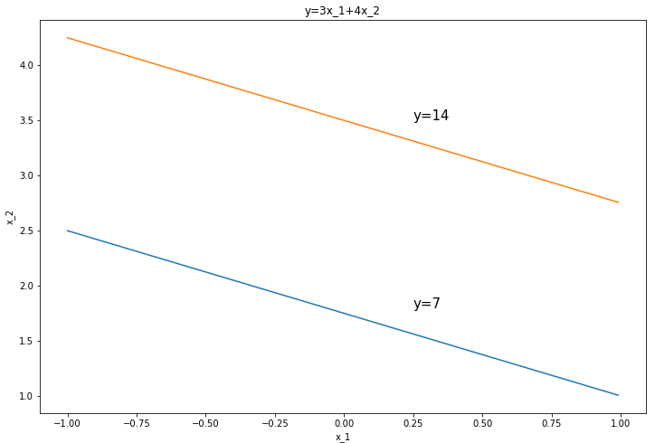
import numpy as np
import matplotlib.pyplot as plt
x1 = np.arange(-1,1,0.01)
fig,ax = plt.subplots(figsize=(12,8))
for y in range(7,15,7):
    x2=(y-3*x1)/4

    ax.plot(x1,x2)
plt.xlabel("x_1")
plt.ylabel("x_2")
plt.text(0.25,3.5,'y=14',fontsize=15,)
plt.text(0.25,1.8,'y=7',fontsize=15,)
plt.title("y=3x_1+4x_2")
plt.show()
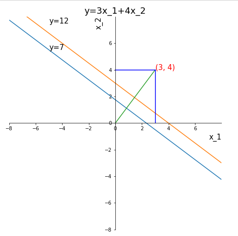
import numpy as np
import matplotlib.pyplot as plt
x1 = np.arange(-10,10,0.01)
fig,ax = plt.subplots(figsize=(12,8))
ax.set_aspect(1)#让x,y轴单位距离一致
for y in range(7,15,5):
    x2=(y-3*x1)/4

    ax.plot(x1,x2)

ax.plot([0,3],[0,4])
ax.plot([0,3],[4,4],color='b')
ax.plot([3,3],[0,4],color='b')
#去掉边框
ax.spines['right'].set_color('none')
ax.spines['top'].set_color('none')
# 设置中心的为(0,0)的坐标轴
ax.spines['bottom'].set_position(('data', 0))  # 指定 data 设置的bottom(也就是指定的x轴)绑定到y轴的0这个点上
ax.spines['left'].set_position(('data', 0))
plt.xlabel("x_1",fontsize=15,loc='right')
plt.ylabel("x_2",fontsize=15,loc='top')
#刻度线
xticks=list(range(-8,8,2))
plt.xticks(xticks)
yticks=list(range(-8,8,2))
plt.yticks(yticks)
#坐标轴范围
plt.xlim((-8,8))
plt.ylim((-8,8))
plt.text(3,4,(3,4),fontsize=15,color='r')
plt.text(-5.0,7.5,'y=12',fontsize=15,)
plt.text(-5.0,5.5,'y=7',fontsize=15,)
plt.title("y=3x_1+4x_2",fontsize=18)
plt.show()
- 通用
import matplotlib.pyplot as plt
#中文问题
plt.rcParams['font.sans-serif'] = ['SimHei']
plt.rcParams['axes.unicode_minus'] = False
# 显示图片
from PIL import image
plt.imshow(img)
plt.show()
'''
img:
	image.open(path)#PIL读取方式为rgb
	#opencv读取方式为bgr
	cv.cvtColor(cv.imread(path), cv.COLOR_BGR2RGB)

'''
#设置全局变量
plt.rcParams
plt.rcParams['font.sans-serif']=['SimHei']#正常显示中文
plt.rcParams['axes.unicode_minus']=False # 用来正常显示负号

# 刻度大小
plt.rcParams['axes.labelsize']=16
# 线的粗细
plt.rcParams['lines.linewidth']=17.5

plt.rcParams['xtick.labelsize']=14 # x轴标签数字大小
plt.rcParams['ytick.labelsize']=14 # y轴标签数字大小

#无plt.rcParams['title.fontsize'] plt.title('x',fontsize=)中设置
plt.rcParams['legend.fontsize']=14 #图例字体大小
# 图大小
#定义一个画布
plt.figure()
'''
plt.figure(num=5,figsize=(4,4)) 画布大小
num指定figure画布的编号,figsize指定画布的大小
'''
'''
一个画布上有多个子图,两种方式,多用第二种
'''

#第一种 subplots,一次创建多个子图,fig是画布对象,ax是子图对象array,当row_num>1 and col_num>1时,ax是个二维array,ax[0]是第一行画布
fig,ax=plt.subplots(row_num/2,col_num/3,figsize=(20,10))
ax=fig.subplots(row_num,col_num,figsize=(20,10))
'''
ax[1][2]=ax[1,2]
ax2=ax[1,2]
ax2.hist()#第二行第三个子图使用直方图
ax2.set_xlabel('设置子图x轴名字')
ax2.set_ylabel('设置子图y轴名字')
ax2.set_title('设置子图标题')
'''
#第二种subplot,当在其中一个子图中画sns图时,使用一次创建一个子图,画布从左到右从上到下的第3个
plt.figure(figsize=(10,10))
ax1=plt.subplot(2,3,1)==plt.subplot(231)#两行三列个子图,第1个子图
plt.plot(x_arr,y_arr,color="b",lines="--")
ax.xlabel()
ax.ylabel()
ax2=plt.subplot(2,3,2)==plt.subplot(232)#两行三列个子图,第2个子图
plt.plot(x_arr2,y_arr2,color="r",lines="--")
ax2.xlabel()
ax2.ylabel()
'''
如果想要设置画布大小的话
plt.figure(figsize=(x,y))
plt.subplot(122)
plt.plot()
#设置坐标轴名称
plt.xlabel('x label')
plt.ylabel('y label')
plt.title('title')

# sns配套使用
plt.subplot(122)
sns.violinplot(x='列名1',y='列名2',data=df)
'''
#设置坐标轴范围
plt.xlim((0,11))
plt.ylim((0.85,1))
plt.rcParams['axes.unicode_minus']=False # 用来正常显示负号
#设置刻度字体大小
plt.xticks(fontsize=15)
plt.yticks(fontsize=15)
#设置连续数字的坐标轴精度
xticks=list(range(0,11,1))#[0,1,.,10]
plt.xticks(xticks)
#设置不连续数字,或者文字的坐标轴
xticks=['cws',1,'pos',2]
plt.xticks(list(range(len(xticks))),xticks)
#设置坐标轴名称,和字体大小
plt.rcParams['font.sans-serif']=['SimHei']#正常显示中文
plt.xlabel('x label'fontsize=)
plt.ylabel('y label'fontsize=)
plt.title('title', fontsize=)
#显示图
plt.show()
#保存画布
plt.savefig('路径')
-
jupyter notebook
%matplotlib inline#添加该行
柱状图

nums=df.category.value_counts(sort=False).values
plt.figure(figsize=(10,10))
#中文
plt.rcParams['font.sans-serif'] = ['SimHei']
plt.rcParams['axes.unicode_minus'] = False
colors=['#1f77b4', '#ff7f0e', 'gray','r','g','b']
plt.bar(label_arr, df.category.value_counts(sort=False).values,color=colors)
plt.xticks(fontsize=15)
plt.yticks(fontsize=15)
plt.title("瑕疵数量统计",fontsize=20)
for x,y in enumerate(nums):
    plt.text(x,y+100,'%s' %y,ha='center',fontsize=15)
plt.show()
折线图
import matplotlib.pyplot as plt
x=[]#表x坐标轴
labels=[]#每个颜色的折线都代表什么
colors=['red', 'blue', 'black', 'green']#多条折线颜色不同
X=[[],[],[]]#多维数组,一个[]是一根线的数据
for i in range(len(X)):
	plt.plot(x, X[i], c=colors[i], label=labels[i],marker='.')
	#markers=['.','v','>','<','^','o','*']等 标记每个点
    #没有color的话,也会默认给多条线分别不同的颜色
    #label是线的名字


plt.plot(x,y,'bo',label='xx')#'bo'为蓝色圆点,'b'为蓝色实线,
#设置坐标轴范围
plt.xlim(0,11)
plt.ylim(0.85,1)
#设置坐标轴精度
xticks=list(range(0,11,1))#[0,1,.,10]
plt.xticks(xticks)
#设置坐标轴名称
plt.xlabel=('x label')
plt.ylabel=('y label')
plt.title('title')

plt.legend(loc='best',fontsize=)##自适应方式放置多个图例(eg:每个颜色的折线都代表啥意思),默认放在  fontsize图例字体大小
'''
'best'         : 0,
'upper right'  : 1,
'upper left'   : 2,
'lower left'   : 3,
'lower right'  : 4,
'right'        : 5,
'center left'  : 6,
'center right' : 7,
'lower center' : 8,
'upper center' : 9,
'center'       : 10,
'''
#显示图
plt.show()
散点图
plt.scatter(array_like_1,array_like_2,alpha=1,c='blue',marker='.')
'''
alpha为透明度,为0.6,颜色浅一些,更好看
c:散点图颜色
marker:散点图形状 #markers=['.','v','>','<','^','o','*']等 标记每个点
'''
plt.show()

不能直接df[['x','y']].scatter()
直方图 hist
plt.hist(array_like/Series,bin=20,color='darkorange')#划分多少个区间

se.hist(bins=100)
se.plot('hist',bins=100)
sns.distplot(se) 带有外轮廓线
显示特征的分布情况(数字型为直方图,非数字型为条形图)
distribution(df1, graph_num=10, graph_num_per_row=5)
# 特征的分布图(直方图or条形图)
def distribution(df, graph_num, graph_num_per_row):
    '''
    只使用取值在2~49的特征,特征最多使用graph_num个

    df:读取的文件
    nGraphShown:最多画几个特征的分布图
    nGraphPerRow:每行画几个图
    '''
    #Series,index为特征,值为该特征有几个取值
    nunique = df.nunique()
    #获取取值个数为2~49的所有特征的df
    df = df[[col for col in df if nunique[col] > 1 and nunique[col] < 50]] # For displaying purposes, pick columns that have between 1 and 50 unique values
    #nRow样本数,ncol特征数
    nRow, nCol = df.shape
   # 取值个数为2~49的所有特征名的list
    columnNames = list(df)

    #要画几个特征的分布图
    real_cols=min(nCol,graph_num)
    #int(4.6)->4 几行图  10+5-1/5=2.8
    nGraphRow = int( (real_cols + graph_num_per_row - 1) / graph_num_per_row )

    plt.figure(figsize = (6 * graph_num_per_row, 6 * nGraphRow), dpi = 80, facecolor = 'w', edgecolor = 'k')
    for i in range(real_cols):
        plt.subplot(nGraphRow, graph_num_per_row, i + 1)
        columnDf = df.iloc[:, i]#是个Series
        if (not np.issubdtype(type(columnDf[0]), np.number)):#非数字型
            #每个取值各有几个,返回Series
            valueCounts = columnDf.value_counts()
            valueCounts.plot.bar()#条形图
        else: #是数字型号
            columnDf.hist()#直方图
        plt.ylabel('counts')
        plt.xticks(rotation = 90)
        plt.title(f'{columnNames[i]} (column {i})')
    plt.tight_layout(pad = 1.0, w_pad = 1.0, h_pad = 1.0)
    plt.show()
显示特征的相关性
简单的:
plt.figure(figsize=(18,9))
corr=df.corr()#特征已经挑出来了
sns.heatmap(corr)
plt.show()

#复杂点的
corr(df1, fig_size=(8,8),file_name='structures_bond.csv')

# Correlation matrix
#相关性图
def corr(df, fig_size, file_name):
    '''
    使用取值个数>1的特征

    graph_width:该图的宽度
    '''
    #去掉存在缺失值Nan的列
    df = df.dropna(axis=0, how='any')

    #保留取值超过1个的特征
    df = df[[col for col in df if df[col].nunique() > 1]] # keep columns where there are more than 1 unique values
    if df.shape[1] < 2:#若取值超过一个的特征只有一个
        print(f'No correlation plots shown: The number of non-NaN or constant columns ({df.shape[1]}) is less than 2')
        return #返回None
    corr = df.corr()
    plt.figure( figsize=fig_size, dpi=80, facecolor='w', edgecolor='k')
    corrMat = plt.matshow(corr, fignum = 1)
    plt.xticks(range(len(corr.columns)), corr.columns, rotation=90)
    plt.yticks(range(len(corr.columns)), corr.columns)
    plt.gca().xaxis.tick_bottom()
    plt.colorbar(corrMat)
    plt.title(f'Correlation Matrix for {file_name}', fontsize=15)
    plt.show()
特征的散点图和密度图(对角线为特征的密度图【可选直方图】,其他为两个特征的散点图)
scatter_density(df1, fig_size=(20,20), text_size=10)

# 散点图和密度图
def scatter_density(df, fig_size, text_size):
    '''
    最多使用9个特征
    '''
    #保留数字型
    df = df.select_dtypes(include =[np.number]) # keep only numerical columns

    df = df.dropna(axis=1, how='any')
    #保留取值超过1个的特征
    df = df[[col for col in df if df[col].nunique() > 1]]
    columnNames = list(df)
    if len(columnNames) > 10: # reduce the number of columns for matrix inversion of kernel density plots
        #最多保留9个特征
        columnNames = columnNames[:10]
    df = df[columnNames]
    ax = pd.plotting.scatter_matrix(df, alpha=0.75, figsize=fig_size, diagonal='kde')
    '''
    alpha为透明度
    diagonal:对角线是 直方图'hist‘,还是核密度图 'kde'
    hist_kwds:传递给hist函数 {'bins':20}
    '''
    corrs = df.corr().values
    for i, j in zip(*plt.np.triu_indices_from(ax, k = 1)):
        ax[i, j].annotate('Corr. coef = %.3f' % corrs[i, j], (0.8, 0.2), xycoords='axes fraction', ha='center', va='center', size=text_size)
    plt.suptitle('Scatter and Density Plot')
    plt.show()
不同类别的target的分布情况
unique = train_df.type.unique()
# x轴标签大小
plt.rcParams['xtick.labelsize']=20
# y轴标签大小
plt.rcParams['ytick.labelsize']=20
print('类别数量:',len(unique))#2*4==8个类别
print('** 不同类别的分布 **')
plt.figure(figsize=(8*4,8*2))
for i in range(len(unique)):
    plt.subplot(2,4,i+1)
    df[df.type==unique[i]].target.hist(color='darkorange')
    plt.title(unique[i],fontsize=20)#标题字体大小
plt.show()

#若某个类别在取值上有明显的断层,可以在另一个特征的帮助下,将其再分子类
保存参数
#保存字典
np.save('dic.npy',dic)
#加载,返回字典
np.load('d.npy',allow_pickle=True).item()


 1587
1587

 被折叠的 条评论
为什么被折叠?
被折叠的 条评论
为什么被折叠?
 到【灌水乐园】发言


