


堆和堆的应用:堆排序和优先队列
1.堆
堆(Heap)是一种重要的数据结构,是实现优先队列(Priority Queues)
首选的数据结构。由于堆有很多种变体,包括二项式堆、斐波那契堆等,但是这里只考虑最常见的就是二叉堆(以下简称堆)。
堆是一棵满足一定性质的二叉树,具体的讲堆具有如下性质:父节点的键值总是不大于它的孩子节点的键值(小顶堆), 堆可以分为小顶堆和大顶堆,这里以小顶堆为例,其主要包含的操作有:
- insert()
- extractMin
- peek(findMin)
- delete(i)
由于堆是一棵形态规则的二叉树,因此堆的父节点和孩子节点存在如下关系:
设父节点的编号为
i, 则其左孩子节点的编号为2*i+1, 右孩子节点的编号为2*i+2
设孩子节点的编号为i, 则其父节点的编号为(i-1)/2
由于二叉树良好的形态已经包含了父节点和孩子节点的关系信息,因此就可以不使用链表而简单的使用数组来存储堆。
要实现堆的基本操作,涉及到的两个关键的函数
- siftUp(i, x) : 将位置i的元素x向上调整,以满足堆得性质,常常是用于insert后,用于调整堆;
- siftDown(i, x):同理,常常是用于delete(i)后,用于调整堆;
具体的操作如下:
private void siftUp(int i) {
    int key = nums[i];
    for (; i > 0;) {
        int p = (i - 1) >>> 1;
        if (nums[p] <= key)
            break;
        nums[i] = nums[p];
        i = p;
    }
    nums[i] = key;
}- 1
- 2
- 3
- 4
- 5
- 6
- 7
- 8
- 9
- 10
- 11
private void siftDown(int i) {
        int key = nums[i];
        for (;i < nums.length / 2;) {
            int child = (i << 1) + 1;
            if (child + 1 < nums.length && nums[child] > nums[child+1])
                child++;
            if (key <= nums[child])
                break;
            nums[i] = nums[child];
            i = child;
        }
        nums[i] = key;
}- 1
- 2
- 3
- 4
- 5
- 6
- 7
- 8
- 9
- 10
- 11
- 12
- 13
可以看到siftUp和siftDown不停的在父节点和子节点之间比较、交换;在不超过logn的时间复杂度就可以完成一次操作。
有了这两个基本的函数,就可以实现上述提及的堆的基本操作。
首先是如何建堆,实现建堆操作有两个思路:
- 一个是不断地
insert(insert后调用的是siftUp) - 另一个将原始数组当成一个需要调整的堆,然后自底向上地
在每个位置i调用siftDown(i),完成后我们就可以得到一个满足堆性质的堆。这里考虑后一种思路:
通常堆的insert操作是将元素插入到堆尾,由于新元素的插入可能违反堆的性质,因此需要调用siftUp操作自底向上调整堆;堆移除堆顶元素操作是将堆顶元素删除,然后将堆最后一个元素放置在堆顶,接着执行siftDown操作,同理替换堆顶元素也是相同的操作。
建堆
// 建立小顶堆
private void buildMinHeap(int[] nums) {
    int size = nums.length;
    for (int j = size / 2 - 1; j >= 0; j--)
        siftDown(nums, j, size);
}
- 1
- 2
- 3
- 4
- 5
- 6
- 7
那么建堆操作的时间复杂度是多少呢?答案是O(n)。虽然siftDown的操作时间是logn,但是由于高度在递减的同时,每一层的节点数量也在成倍减少,最后通过数列错位相减可以得到时间复杂度是O(n)。
extractMin
由于堆的固有性质,堆的根便是最小的元素,因此peek操作就是返回根nums[0]元素即可;
若要将nums[0]删除,可以将末尾的元素nums[n-1]覆盖nums[0],然后将堆得size = size-1,调用siftDown(0)调整堆。时间复杂度为logn。
peek
同上
delete(i)
删除堆中位置为i的节点,涉及到两个函数siftUp和siftDown,时间复杂度为logn,具体步骤是,
- 将元素last覆盖元素i,然后siftDown
- 检查是否需要siftUp
注意到堆的删除操作,如果是删除堆的根节点,则不用考虑执行siftUp的操作;若删除的是堆的非根节点,则要视情况决定是siftDown还是siftUp操作,两个操作是互斥的。
public int delete(int i) {
    int key = nums[i];
    //将last元素移动过来,先siftDown; 再视情况考虑是否siftUp
    int last = nums[i] = nums[size-1];
    size--;
    siftDown(i);
    //check #i的node的键值是否确实发生改变(是否siftDown操作生效),若发生改变,则ok,否则为确保堆性质,则需要siftUp
    if (i < size && nums[i] == last) {
        System.out.println("delete siftUp");
        siftUp(i);
    }
     return key;
}
- 1
- 2
- 3
- 4
- 5
- 6
- 7
- 8
- 9
- 10
- 11
- 12
- 13
- 14
- 15
case 1 :
删除中间节点i21,将最后一个节点复制过来;

由于没有进行siftDown操作,节点i的值仍然为6,因此为确保堆的性质,执行siftUp操作;

case 2
删除中间节点i,将值为11的节点复制过来,执行siftDown操作; 
由于执行siftDown操作后,节点i的值不再是11,因此就不用再执行siftUp操作了,因为堆的性质在siftDown操作生效后已经得到了保持。

可以看出,堆的基本操作都依赖于两个核心的函数siftUp和siftDown;较为完整的Heap代码如下:
class Heap {
    private final static int N = 100; //default size
    private int[] nums;
    private int size;

    public Heap(int[] nums) {
        this.nums = nums;
        this.size = nums.length;
        heapify(this.nums);
    }

    public Heap() {
        this.nums = new int[N];
    }

    /**
     * heapify an array, O(n)
     * @param nums An array to be heapified.
     */
    private void heapify(int[] nums) {
        for (int j = (size - 1) >> 1; j >= 0; j--)
            siftDown(j);
    }

    /**
     * append x to heap
     * O(logn)
     * @param x
     * @return
     */
    public int insert(int x) {
        if (size >= this.nums.length)
            expandSpace();
        size += 1;
        nums[size-1] = x;
        siftUp(size-1);
        return x;
    }

    /**
     * delete an element located in i position.
     * O(logn)
     * @param i
     * @return
     */
    public int delete(int i) {
        rangeCheck(i);
        int key = nums[i];
        //将last元素覆盖过来,先siftDown; 再视情况考虑是否siftUp;
        int last = nums[i] = nums[size-1];
        size--;
        siftDown(i);
        //check #i的node的键值是否确实发生改变,若发生改变,则ok,否则为确保堆性质,则需要siftUp;
        if (i < size && nums[i] == last)
            siftUp(i);
        return key;
    }

    /**
     * remove the root of heap, return it's value, and adjust heap to maintain the heap's property.
     * O(logn)
     * @return
     */
    public int extractMin() {
        rangeCheck(0);
        int key = nums[0], last = nums[size-1];
        nums[0] = last;
        size--;
        siftDown(0);
        return key;
    }
    /**
     * return an element's index, if not exists, return -1;
     * O(n)
     * @param x
     * @return
     */
    public int search(int x) {
        for (int i = 0; i < size; i++)
            if (nums[i] == x)
                return i;
        return -1;
    }
    /**
     * return but does not remove the root of heap.
     * O(1)
     * @return
     */
    public int peek() {
        rangeCheck(0);
        return nums[0];
    }

    private void siftUp(int i) {
        int key = nums[i];
        for (; i > 0;) {
            int p = (i - 1) >>> 1;
            if (nums[p] <= key)
                break;
            nums[i] = nums[p];
            i = p;
        }
        nums[i] = key;
    }

    private void siftDown(int i) {
        int key = nums[i];
        for (;i < size / 2;) {
            int child = (i << 1) + 1;
            if (child + 1 < size && nums[child] > nums[child+1])
                child++;
            if (key <= nums[child])
                break;
            nums[i] = nums[child];
            i = child;
        }
        nums[i] = key;
    }

    private void rangeCheck(int i) {
        if (!(0 <= i && i < size))
            throw new RuntimeException("Index is out of boundary");
    }

    private void expandSpace() {
        this.nums = Arrays.copyOf(this.nums, size * 2);
    }

    @Override
    public String toString() {
        // TODO Auto-generated method stub
        StringBuilder sb = new StringBuilder();
        sb.append("[");
        for (int i = 0; i < size; i++)
            sb.append(String.format((i != 0 ? ", " : "") + "%d", nums[i]));
        sb.append("]\n");
        return sb.toString();
    }
}- 1
- 2
- 3
- 4
- 5
- 6
- 7
- 8
- 9
- 10
- 11
- 12
- 13
- 14
- 15
- 16
- 17
- 18
- 19
- 20
- 21
- 22
- 23
- 24
- 25
- 26
- 27
- 28
- 29
- 30
- 31
- 32
- 33
- 34
- 35
- 36
- 37
- 38
- 39
- 40
- 41
- 42
- 43
- 44
- 45
- 46
- 47
- 48
- 49
- 50
- 51
- 52
- 53
- 54
- 55
- 56
- 57
- 58
- 59
- 60
- 61
- 62
- 63
- 64
- 65
- 66
- 67
- 68
- 69
- 70
- 71
- 72
- 73
- 74
- 75
- 76
- 77
- 78
- 79
- 80
- 81
- 82
- 83
- 84
- 85
- 86
- 87
- 88
- 89
- 90
- 91
- 92
- 93
- 94
- 95
- 96
- 97
- 98
- 99
- 100
- 101
- 102
- 103
- 104
- 105
- 106
- 107
- 108
- 109
- 110
- 111
- 112
- 113
- 114
- 115
- 116
- 117
- 118
- 119
- 120
- 121
- 122
- 123
- 124
- 125
- 126
- 127
- 128
- 129
- 130
- 131
- 132
- 133
- 134
- 135
- 136
- 137
- 138
- 139
2.堆的应用:堆排序
运用堆的性质,我们可以得到一种常用的、稳定的、高效的排序算法————堆排序。堆排序的时间复杂度为O(n*log(n)),空间复杂度为O(1),堆排序的思想是:
对于含有n个元素的无序数组nums, 构建一个堆(这里是小顶堆)heap,然后执行extractMin得到最小的元素,这样执行n次得到序列就是排序好的序列。
如果是降序排列则是小顶堆;否则利用大顶堆。
Trick
由于extractMin执行完毕后,最后一个元素last已经被移动到了root,因此可以将extractMin返回的元素放置于最后,这样可以得到sort in place的堆排序算法。
具体操作如下:
int[] n = new int[] {1,9,5,6,8,3,1,2,5,9,86};
Heap h = new Heap(n);
for (int i = 0; i < n.length; i++)
    n[n.length-1-i] = h.extractMin();
- 1
- 2
- 3
- 4
- 5
当然,如果不使用前面定义的heap,则可以手动写堆排序,由于堆排序设计到建堆和extractMin, 两个操作都公共依赖于siftDown函数,因此我们只需要实现siftDown即可。(trick:由于建堆操作可以采用siftUp或者siftDown,而extractMin是需要siftDown操作,因此取公共部分,则采用siftDown建堆)。
这里便于和前面统一,采用小顶堆数组进行降序排列。
public void heapSort(int[] nums) {
        int size = nums.length;
        buildMinHeap(nums);
        while (size != 0) {
            // 交换堆顶和最后一个元素
            int tmp = nums[0];
            nums[0] = nums[size - 1];
            nums[size - 1] = tmp;
            size--;
            siftDown(nums, 0, size);
        }
    }

    // 建立小顶堆
    private void buildMinHeap(int[] nums) {
        int size = nums.length;
        for (int j = size / 2 - 1; j >= 0; j--)
            siftDown(nums, j, size);
    }

    private void siftDown(int[] nums, int i, int newSize) {
        int key = nums[i];
        while (i < newSize >>> 1) {
            int leftChild = (i << 1) + 1;
            int rightChild = leftChild + 1;
            // 最小的孩子,比最小的孩子还小
            int min = (rightChild >= newSize || nums[leftChild] < nums[rightChild]) ? leftChild : rightChild;
            if (key <= nums[min])
                break;
            nums[i] = nums[min];
            i = min;
        }
        nums[i] = key;
    }
- 1
- 2
- 3
- 4
- 5
- 6
- 7
- 8
- 9
- 10
- 11
- 12
- 13
- 14
- 15
- 16
- 17
- 18
- 19
- 20
- 21
- 22
- 23
- 24
- 25
- 26
- 27
- 28
- 29
- 30
- 31
- 32
- 33
- 34
- 35
- 36
3.堆的应用:优先队列
优先队列是一种抽象的数据类型,它和堆的关系类似于,List和数组、链表的关系一样;我们常常使用堆来实现优先队列,因此很多时候堆和优先队列都很相似,它们只是概念上的区分。
优先队列的应用场景十分的广泛:
常见的应用有:
- Dijkstra’s algorithm(单源最短路问题中需要在邻接表中找到某一点的最短邻接边,这可以将复杂度降低。)
- Huffman coding(贪心算法的一个典型例子,采用优先队列构建最优的前缀编码树(prefixEncodeTree))
- Prim’s algorithm for minimum spanning tree
- Best-first search algorithms
这里简单介绍上述应用之一:Huffman coding。
Huffman编码是一种变长的编码方案,对于每一个字符,所对应的二进制位串的长度是不一致的,但是遵守如下原则:
- 出现频率高的字符的二进制位串的长度小
- 不存在一个字符c的二进制位串s是除c外任意字符的二进制位串的前缀
遵守这样原则的Huffman编码属于变长编码,可以无损的压缩数据,压缩后通常可以节省20%-90%的空间,具体压缩率依赖于数据的固有结构。
Huffman编码的实现就是要找到满足这两种原则的 字符-二进制位串 对照关系,即找到最优前缀码的编码方案(前缀码:没有任何字符编码后的二进制位串是其他字符编码后位串的前缀)。
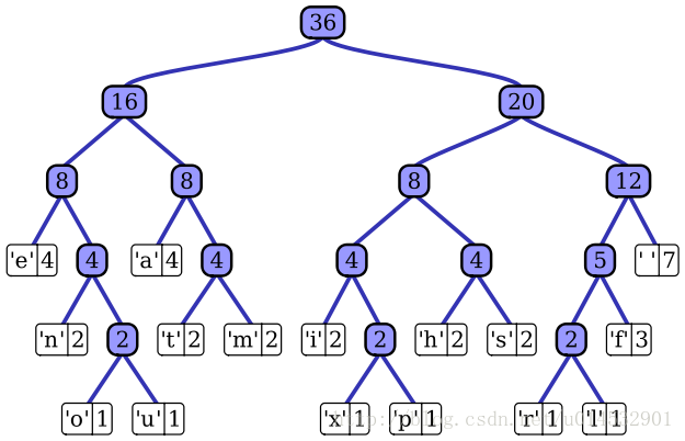
这里我们需要用到二叉树来表达最优前缀码,该树称为最优前缀码树
一棵最优前缀码树看起来像这样:
算法思想:用一个属性为freqeunce关键字的最小优先队列Q,将当前最小的两个元素x,y合并得到一个新元素z(z.frequence = x.freqeunce + y.frequence),
然后插入到优先队列中Q中,这样执行n-1次合并后,得到一棵最优前缀码树(这里不讨论算法的证明)。
一个常见的构建流程如下:
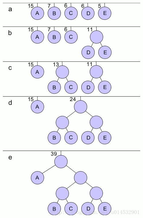
树中指向某个节点左孩子的边上表示位0,指向右孩子的边上的表示位1,这样遍历一棵最优前缀码树就可以得到对照表。
import java.util.Comparator;
import java.util.HashMap;
import java.util.Map;
import java.util.PriorityQueue;

/**
 *
 *                            root
 *                            /   \
 *                    --------- ----------
 *                    |c:freq | | c:freq |
 *                    --------- ----------
 *
 *
 */
public class HuffmanEncodeDemo {

    public static void main(String[] args) {
        // TODO Auto-generated method stub
        Node[] n = new Node[6];
        float[] freq = new float[] { 9, 5, 45, 13, 16, 12 };
        char[] chs = new char[] { 'e', 'f', 'a', 'b', 'd', 'c' };
        HuffmanEncodeDemo demo = new HuffmanEncodeDemo();
        Node root = demo.buildPrefixEncodeTree(n, freq, chs);
        Map<Character, String> collector = new HashMap<>();
        StringBuilder sb = new StringBuilder();
        demo.tranversalPrefixEncodeTree(root, collector, sb);
        System.out.println(collector);
        String s = "abcabcefefefeabcdbebfbebfbabc";
        StringBuilder sb1 = new StringBuilder();
        for (char c : s.toCharArray()) {
            sb1.append(collector.get(c));
        }
        System.out.println(sb1.toString());
    }

    public Node buildPrefixEncodeTree(Node[] n, float[] freq, char[] chs) {
        PriorityQueue<Node> pQ = new PriorityQueue<>(new Comparator<Node>() {
            public int compare(Node o1, Node o2) {
                return o1.item.freq > o2.item.freq ? 1 : o1.item.freq == o2.item.freq ? 0 : -1;
            };
        });
        Node e = null;
        for (int i = 0; i < chs.length; i++) {
            n[i] = e = new Node(null, null, new Item(chs[i], freq[i]));
            pQ.add(e);
        }

        for (int i = 0; i < n.length - 1; i++) {
            Node x = pQ.poll(), y = pQ.poll();
            Node z = new Node(x, y, new Item('$', x.item.freq + y.item.freq));
            pQ.add(z);
        }
        return pQ.poll();
    }

    /**
     * tranversal
     * @param root
     * @param collector
     * @param sb
     */
    public void tranversalPrefixEncodeTree(Node root, Map<Character, String> collector, StringBuilder sb) {
        // leaf node
        if (root.left == null && root.right == null) {
            collector.put(root.item.c, sb.toString());
            return;
        }
        Node left = root.left, right = root.right;
        tranversalPrefixEncodeTree(left, collector, sb.append(0));
        sb.delete(sb.length() - 1, sb.length());
        tranversalPrefixEncodeTree(right, collector, sb.append(1));
        sb.delete(sb.length() - 1, sb.length());
    }

}

class Node {
    public Node left, right;
    public Item item;

    public Node(Node left, Node right, Item item) {
        super();
        this.left = left;
        this.right = right;
        this.item = item;
    }

}

class Item {
    public char c;
    public float freq;

    public Item(char c, float freq) {
        super();
        this.c = c;
        this.freq = freq;
    }
}
- 1
- 2
- 3
- 4
- 5
- 6
- 7
- 8
- 9
- 10
- 11
- 12
- 13
- 14
- 15
- 16
- 17
- 18
- 19
- 20
- 21
- 22
- 23
- 24
- 25
- 26
- 27
- 28
- 29
- 30
- 31
- 32
- 33
- 34
- 35
- 36
- 37
- 38
- 39
- 40
- 41
- 42
- 43
- 44
- 45
- 46
- 47
- 48
- 49
- 50
- 51
- 52
- 53
- 54
- 55
- 56
- 57
- 58
- 59
- 60
- 61
- 62
- 63
- 64
- 65
- 66
- 67
- 68
- 69
- 70
- 71
- 72
- 73
- 74
- 75
- 76
- 77
- 78
- 79
- 80
- 81
- 82
- 83
- 84
- 85
- 86
- 87
- 88
- 89
- 90
- 91
- 92
- 93
- 94
- 95
- 96
- 97
- 98
- 99
- 100
- 101
输出如下:
{a=0, b=101, c=100, d=111, e=1101, f=1100}
010110001011001101110011011100110111001101010110011110111011011100101110110111001010101100- 1
- 2
4 堆的应用:海量实数中(一亿级别以上)找到TopK(一万级别以下)的数集合。
A:通常遇到找一个集合中的TopK问题,想到的便是排序,因为常见的排序算法例如快排算是比较快了,然后再取出K个TopK数,时间复杂度为
O(nlogn),当n很大的时候这个时间复杂度还是很大的;B:另一种思路就是打擂台的方式,每个元素与K个待选元素比较一次,时间复杂度很高:
O(k*n),此方案明显逊色于前者。
对于一亿数据来说,A方案大约是26.575424*n;
- C:由于我们只需要TopK,因此不需要对所有数据进行排序,可以利用堆得思想,维护一个大小为K的小顶堆,然后依次遍历每个元素
e, 若元素e大于堆顶元素root,则删除root,将e放在堆顶,然后调整,时间复杂度为logK;若小于或等于,则考察下一个元素。这样遍历一遍后,最小堆里面保留的数就是我们要找的topK,整体时间复杂度为O(k+n*logk)约等于O(n*logk),大约是13.287712*n(由于k与n数量级差太多),这样时间复杂度下降了约一半。
A、B、C三个方案中,C通常是优于B的,因为logK通常是小于k的,当K和n的数量级相差越大,这种方式越有效。
以下为具体操作:
import java.io.File;
import java.io.FileNotFoundException;
import java.io.PrintWriter;
import java.io.UnsupportedEncodingException;
import java.util.Arrays;
import java.util.Scanner;
import java.util.Set;
import java.util.TreeSet;
public class TopKNumbersInMassiveNumbersDemo {

    public static void main(String[] args) {
        // TODO Auto-generated method stub
        int[] topK = new int[]{50001,50002,50003,50004,50005};
        genData(1000 * 1000 * 1000, 500, topK);
        long t = System.currentTimeMillis();
        findTopK(topK.length);
        System.out.println(String.format("cost:%fs", (System.currentTimeMillis() - t) * 1.0 / 1000));
    }

    public static void genData(int N, int maxRandomNumer, int[] topK) {
        File f = new File("data.txt");
        int k = topK.length;
        Set<Integer> index = new TreeSet<>();
        for (;;) {
            index.add((int)(Math.random() * N));
            if (index.size() == k)
                break;
        }
        System.out.println(index);
        int j = 0;
        try {
            PrintWriter pW = new PrintWriter(f, "UTF-8");
            for (int i = 0; i < N; i++)
                if(!index.contains(i))
                    pW.println((int)(Math.random() * maxRandomNumer));
                else
                    pW.println(topK[j++]);
            pW.flush();
        } catch (FileNotFoundException e) {
            // TODO Auto-generated catch block
            e.printStackTrace();
        } catch (UnsupportedEncodingException e) {
            // TODO Auto-generated catch block
            e.printStackTrace();
        }
    }

    public static void findTopK(int k) {
        int[] nums = new int[k];
        //read
        File f = new File("data.txt");
        try {
            Scanner scanner = new Scanner(f);
            for (int j = 0;j < k; j++)
                nums[j] = scanner.nextInt();
            heapify(nums);
            //core
            while (scanner.hasNextInt()) {
                int a = scanner.nextInt();
                if (a <= nums[0])
                    continue;
                else {
                    nums[0] = a;
                    siftDown(0, k, nums);
                }
            }
            System.out.println(Arrays.toString(nums));
        } catch (FileNotFoundException e) {
            // TODO Auto-generated catch block
            e.printStackTrace();
        }

    }

    //O(n), minimal heap
    public static void heapify(int[] nums) {
        int size = nums.length;
        for (int j = (size - 1) >> 1; j >= 0; j--)
            siftDown(j, size, nums);
    }

    private static void siftDown(int i, int n, int[] nums) {
        int key = nums[i];
        for (;i < (n >>> 1);) {
            int child = (i << 1) + 1;
            if (child + 1 < n && nums[child] > nums[child+1])
                child++;
            if (key <= nums[child])
                break;
            nums[i] = nums[child];
            i = child;
        }
        nums[i] = key;
    }
}- 1
- 2
- 3
- 4
- 5
- 6
- 7
- 8
- 9
- 10
- 11
- 12
- 13
- 14
- 15
- 16
- 17
- 18
- 19
- 20
- 21
- 22
- 23
- 24
- 25
- 26
- 27
- 28
- 29
- 30
- 31
- 32
- 33
- 34
- 35
- 36
- 37
- 38
- 39
- 40
- 41
- 42
- 43
- 44
- 45
- 46
- 47
- 48
- 49
- 50
- 51
- 52
- 53
- 54
- 55
- 56
- 57
- 58
- 59
- 60
- 61
- 62
- 63
- 64
- 65
- 66
- 67
- 68
- 69
- 70
- 71
- 72
- 73
- 74
- 75
- 76
- 77
- 78
- 79
- 80
- 81
- 82
- 83
- 84
- 85
- 86
- 87
- 88
- 89
- 90
- 91
- 92
- 93
- 94
- 95
ps:大致测试了一下,10亿个数中找到top5需要140秒左右,应该是很快了。
5 总结
- 堆是基于树的满足一定约束的重要数据结构,存在许多变体例如二叉堆、二项式堆、斐波那契堆(很高效)等。
- 堆的几个基本操作都依赖于两个重要的函数
siftUp和siftDown,堆的insert通常是在堆尾插入新元素并siftUp调整堆,而extractMin是在
删除堆顶元素,然后将最后一个元素放置堆顶并调用siftDown调整堆。 - 二叉堆是常用的一种堆,其是一棵二叉树;由于二叉树良好的性质,因此常常采用数组来存储堆。
堆得基本操作的时间复杂度如下表所示:
| heapify | insert | peek | extractMin | delete(i) |
|---|---|---|---|---|
O(n) | O(logn) | O(1) | O(logn) | O(logn) |
- 二叉堆通常被用来实现堆排序算法,堆排序可以sort in place,堆排序的时间复杂度的上界是O(nlogn),是一种很优秀的排序算法。由于存在相同键值的两个元素处于两棵子树中,而两个元素的顺序可能会在后续的堆调整中发生改变,因此堆排序不是稳定的。降序排序需要建立小顶堆,升序排序需要建立大顶堆。
堆是实现抽象数据类型优先队列的一种方式,优先队列有很广泛的应用,例如Huffman编码中使用优先队列利用贪心算法构建最优前缀编码树。
堆的另一个应用就是在海量数据中找到TopK个数,思想是维护一个大小为K的二叉堆,然后不断地比较堆顶元素,判断是否需要执行替换对顶元素的操作,采用
此方法的时间复杂度为n*logk,当k和n的数量级差距很大的时候,这种方式是很有效的方法。

 4301


 扫一扫


 被折叠的 条评论
为什么被折叠?
 到【灌水乐园】发言


