你如何看待不平衡数据

1. 不平衡数据的定义

在分类问题中，类别之间的分布不均匀导致数据的不平衡。比如，针对二分类问题，target取值为0和1，当其中一方（如y=1）的占比远小于另一方（y=0）的时候，就构成了不平衡数据。

那么到底是需要差异多少，才算是失衡呢，根本Google Developer的说法，我们一般可以 把失衡程度分为3个级别 ：

• 轻度：20-40%
• 中度：1-20%
• 极度：<1%

一般来说，失衡样本在构建模型时难以发现问题，甚至可以得到很高的accuracy，为什么呢？假设我们有一个极度失衡的样本，y=1的占比为1%，那么，我们训练的模型，会偏向于把测试集预测为0，从而导致模型整体的预测准确性较高，如果我们只是关注这个指标的话，可能就会被骗了。

3. 处理不平衡数据的理论方法

在我们开始用Python处理失衡样本之前，我们先来了解一下关于处理失衡样本的一些理论知识，前辈们关于这类问题的解决方案，主要包括以下：

• 从数据角度：通过应用一些 欠采样或过采样技术来处理失衡样本。欠采样就是对类别数量多的样本进行抽样，保留类别数量少的样本的全量，使得两类的数量相当；过采样就是对少数类进行多次重复采样，保留类别数量多的样本的全量，使得两类的数量相当。但是，这两类做法也有弊端，欠采样会导致我们丢失一部分的信息，可能包含了一些重要的信息，过采样则会导致分类器容易过拟合。当然，也可以是两种技术的相互结合。
• 从算法角度：算法角度的解决方案就是可以通过对每类的训练实例给予一定权值的调整。比如，在SVM有参分类器中，可以应用grid search（网格搜索）以及交叉验证（cross validation）来优化C以及gamma值。而对于决策树这类的非参数模型，可以通过调整树叶节点上的概率估计从而实现效果优化。
• 数据和算法结合 ：有研究员从数据以及算法的结合角度来看待这类问题，提出了两者结合体的AdaOUBoost（adaptive over-sampling and undersampling boost）算法，这个算法的新颖之处在于自适应地对少数类样本进行过采样，然后对多数类样本进行欠采样，以形成不同的分类器，并根据其准确度将这些子分类器组合在一起从而形成强大的分类器。

4. 常用处理数据不平衡的方法概述

目前主流的方法大致有以下几种（reference只列举出了比较有代表性的）：

• 重采样（re-sampling）：这是解决数据类别不平衡的非常简单而暴力的方法，更具体可以分为两种，对少样本的过采样[1]，或是对多样本的欠采样[2]。当然，这类比较经典的方法一般效果都会欠佳，因为过采样容易overfit到minor classes，无法学到更鲁棒易泛化的特征，往往在非常不平衡的数据上泛化性能会更差；而欠采样则会直接造成major class严重的信息损失，甚至会导致欠拟合的现象发生。
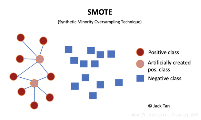
• 数据合成（synthetic samples）：若不想直接重复采样相同样本，一种解决方法是生成和少样本相似的“新”数据。一个最粗暴的方法是直接对少类样本加随机高斯噪声，做data smoothing[3]。此外，此类方法中比较经典的还有SMOTE[4]，其思路简单来讲是对任意选取的一个少类的样本，用K近邻选取其相似的样本，通过对样本的线性插值得到新样本。说道这里不禁想到和mixup[5]很相似，都是在input space做数据插值；当然，对于deep model，也可以在representation上做mixup（manifold-mixup）。基于这个思路，最近也有imbalance的mixup版本出现[6]。
• 重加权（re-weighting）：顾名思义，重加权是对不同类别（甚至不同样本）分配不同权重，主要体现在重加权不同类别的loss来解决长尾分布问题。注意这里的权重可以是自适应的。此类方法的变种有很多，有最简单的按照类别数目的倒数来做加权[7]，按照“有效”样本数加权[8]，根据样本数优化分类间距的loss加权[9]，等等。对于max margin的这类方法，还可以用bayesian对每个样本做uncertainty估计，来refine决策边界[10]。这类方法目前应该是使用的最广泛的，就不贴更多的reference了，可以看一下这个survey paper[3]。
• 迁移学习（transfer learning）：这类方法的基本思路是对多类样本和少类样本分别建模，将学到的多类样本的信息/表示/知识迁移给少类别使用。代表性文章有[11][12]。
• 度量学习（metric learning）：本质上是希望能够学到更好的embedding，对少类附近的boundary/margin更好的建模。有兴趣的同学可以看看[13][14]。这里多说一句，除了采用经典的contrastive/triplet loss的思路，最近火起来的contrastive learning，即做instance-level的discrimination，是否也可以整合到不均衡学习的框架中？
• 元学习/域自适应（meta learning/domain adaptation）：这部分因为文章较少且更新一点，就合并到一起写，最终的目的还是分别对头部和尾部的数据进行不同处理，可以去自适应的学习如何重加权[15]，或是formulate成域自适应问题[16]。
• 解耦特征和分类器（decoupling representation & classifier）：最近的研究发现将特征学习和分类器学习解耦，把不平衡学习分为两个阶段，在特征学习阶段正常采样，在分类器学习阶段平衡采样，可以带来更好的长尾学习结果[17][18]。

1. Samira Pouyanfar, et al. Dynamic sampling in convolutional neural networks for imbalanced data classification.
2. He, H. and Garcia, E. A. Learning from imbalanced data. TKDE, 2008.
3. abP. Branco, L. Torgo, and R. P. Ribeiro. A survey of predictive modeling on imbalanced domains.
4. Chawla, N. V., et al. SMOTE: synthetic minority oversampling technique. JAIR, 2002.
5. mixup: Beyond Empirical Risk Minimization. ICLR 2018.
6. H. Chou et al. Remix: Rebalanced Mixup. 2020.
7. Deep Imbalanced Learning for Face Recognition and Attribute Prediction. TPAMI, 2019.
8. Yin Cui, Menglin Jia, Tsung-Yi Lin, Yang Song, and Serge Belongie. Class-balanced loss based on effective number of samples. In Proceedings of the IEEE Conference on Computer Vision and Pattern Recognition, pages 9268–9277, 2019.
9. Learning Imbalanced Datasets with Label-Distribution-Aware Margin Loss. NeurIPS, 2019.
10. Striking the Right Balance with Uncertainty. CVPR, 2019.
11. Large-scale long-tailed recognition in an open world. CVPR, 2019.
12. Feature transfer learning for face recognition with under-represented data. CVPR, 2019.
13. Range Loss for Deep Face Recognition with Long-Tail. CVPR, 2017.
14. Learning Deep Representation for Imbalanced Classification. CVPR, 2016.
15. Meta-Weight-Net: Learning an Explicit Mapping For Sample Weighting. NeurIPS, 2019.
16. Rethinking Class-Balanced Methods for Long-Tailed Recognition from a Domain Adaptation Perspective. CVPR, 2020.
17. Decoupling representation and classifier for long-tailed recognition. ICLR, 2020.
18. BBN: Bilateral-Branch Network with Cumulative Learning for Long-Tailed Visual Recognition. CVPR, 2020.

5.Python里有什么包可以处理不平衡样本

这里介绍一个很不错的包，叫 imbalanced-learn，大家可以在电脑上安装一下使用。然后，我们就可以实现样本的欠采样、过采样，并且可以利用pipeline的方式来实现两者的结合，十分方便，我们下一节来简单使用一下吧！

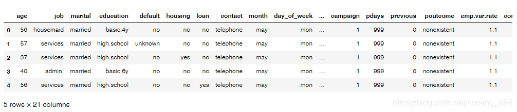
为了更好滴理解，我们引入一个数据集，来自于UCI机器学习存储库的营销活动数据集。(数据集大家可以自己去官网下载：https://archive.ics.uci.edu/ml/machine-learning-databases/00222/。)

我们在完成imblearn库的安装之后，就可以开始简单的操作了（其余更加复杂的操作可以直接看官方文档），以下我会从4方面来演示如何用Python处理失衡样本，分别是：

🌈 1、随机欠采样的实现

🌈 2、使用SMOTE进行过采样

🌈 3、欠采样和过采样的结合（使用pipeline）

🌈 4、如何获取最佳的采样率？

3.1 数据准备

from collections import Counter
from sklearn.model_selection import train_test_split
from sklearn.model_selection import cross_val_score
import pandas as pd
import numpy as np
import warnings
warnings.simplefilter(action='ignore', category=FutureWarning)

from sklearn.svm import SVC
from sklearn.metrics import classification_report, roc_auc_score
from numpy import mean

# 导入数据
df = pd.read_csv('bank-additional-full.csv', ';') # '';'' 为分隔符
df.head()

• 查看数据是否是 失衡样本

可以看出少数类的占比为11.2%，属于中度失衡样本。

df['y'].value_counts()/len(df)
# Out:
# no     0.887346
# yes    0.112654
# Name: y, dtype: float64

• 只保留数值型变量（简单操作）

df = df.loc[:,
['age', 'duration', 'campaign', 'pdays',
       'previous', 'emp.var.rate', 'cons.price.idx',
       'cons.conf.idx', 'euribor3m', 'nr.employed','y']]
# target由 yes/no 转为 0/1
df['y'] = df['y'].apply(lambda x: 1 if x=='yes' else 0)
df['y'].value_counts()

#0    36548
#1     4640
#Name: y, dtype: int64

3.2 随机欠采样的实现

基于 under_sampling.RandomUnderSampler。结果，原先0的样本有21942，欠采样之后就变成了与1一样的数量了（即2770），实现了50%/50%的类别分布。

# 1、随机欠采样的实现
# 导入相关的方法
from imblearn.under_sampling import RandomUnderSampler

# 划分因变量和自变量
X = df.iloc[:,:-1]
y = df.iloc[:,-1]

# 划分训练集和测试集
X_train, X_test, y_train, y_test = train_test_split(X,y,test_size=0.40)

# 统计当前的类别占比情况
print("Before undersampling: ", Counter(y_train))

# 调用方法进行欠采样
undersample = RandomUnderSampler(sampling_strategy='majority')

# 获得欠采样后的样本
X_train_under, y_train_under = undersample.fit_resample(X_train, y_train)

# 统计欠采样后的类别占比情况
print("After undersampling: ", Counter(y_train_under))

# 调用支持向量机算法 SVC
model=SVC()

clf = model.fit(X_train, y_train)
pred = clf.predict(X_test)
print("ROC AUC score for original data: ", roc_auc_score(y_test, pred))

clf_under = model.fit(X_train_under, y_train_under)
pred_under = clf_under.predict(X_test)
print("ROC AUC score for undersampled data: ", roc_auc_score(y_test, pred_under))

# Output：
#Before undersampling:  Counter({0: 21942, 1: 2770})
#After undersampling:  Counter({0: 2770, 1: 2770})
#ROC AUC score for original data:  0.603521152028
#ROC AUC score for undersampled data:  0.829234085179

3.3 使用SMOTE进行过采样

过采样技术中，SMOTE被认为是最为流行的数据采样算法之一，它是基于随机过采样算法的一种改良版本，由于随机过采样只是采取了简单复制样本的策略来进行样本的扩增，这样子会导致一个比较直接的问题就是过拟合。因此，SMOTE的基本思想就是对少数类样本进行分析并合成新样本添加到数据集中。

算法流程如下：

• (1)对于少数类中每一个样本x，以欧氏距离为标准计算它到少数类样本集中所有样本的距离，得到其k近邻。
• (2)根据样本不平衡比例设置一个采样比例以确定采样倍率N，对于每一个少数类样本x，从其k近邻中随机选择若干个样本，假设选择的近邻为xn。
• (3)对于每一个随机选出的近邻xn，分别与原样本按照如下的公式构建新的样本。
  

# 2、使用SMOTE进行过采样
# 导入相关的方法
from imblearn.over_sampling import SMOTE

# 划分因变量和自变量
X = df.iloc[:,:-1]
y = df.iloc[:,-1]

# 划分训练集和测试集
X_train, X_test, y_train, y_test = train_test_split(X,y,test_size=0.40)

# 统计当前的类别占比情况
print("Before oversampling: ", Counter(y_train))

# 调用方法进行过采样
SMOTE = SMOTE()

# 获得过采样后的样本
X_train_SMOTE, y_train_SMOTE = SMOTE.fit_resample(X_train, y_train)

# 统计过采样后的类别占比情况
print("After oversampling: ",Counter(y_train_SMOTE))

# 调用支持向量机算法 SVC
model=SVC()

clf = model.fit(X_train, y_train)
pred = clf.predict(X_test)
print("ROC AUC score for original data: ", roc_auc_score(y_test, pred))

clf_SMOTE= model.fit(X_train_SMOTE, y_train_SMOTE)
pred_SMOTE = clf_SMOTE.predict(X_test)
print("ROC AUC score for oversampling data: ", roc_auc_score(y_test, pred_SMOTE))

# Output：
#Before oversampling:  Counter({0: 21980, 1: 2732})
#After oversampling:  Counter({0: 21980, 1: 21980})
#ROC AUC score for original data:  0.602555700614
#ROC AUC score for oversampling data:  0.844305732561

3.4 欠采样和过采样的结合（使用pipeline）

那如果我们需要同时使用过采样以及欠采样，那该怎么做呢？其实很简单，就是使用 pipeline来实现。

#  3、欠采样和过采样的结合（使用pipeline）
# 导入相关的方法
from imblearn.over_sampling import SMOTE
from imblearn.under_sampling import RandomUnderSampler
from imblearn.pipeline import Pipeline

# 划分因变量和自变量
X = df.iloc[:,:-1]
y = df.iloc[:,-1]

#  定义管道
model = SVC()
over = SMOTE(sampling_strategy=0.4)
under = RandomUnderSampler(sampling_strategy=0.5)
steps = [('o', over), ('u', under), ('model', model)]
pipeline = Pipeline(steps=steps)

# 评估效果
scores = cross_val_score(pipeline, X, y, scoring='roc_auc', cv=5, n_jobs=-1)
score = mean(scores)
print('ROC AUC score for the combined sampling method: %.3f' % score)

# Output：
#ROC AUC score for the combined sampling method: 0.937

3.5 如何获取最佳的采样率？

在上面的栗子中，我们都是默认经过采样变成50：50，但是这样子的采样比例并非最优选择，因此我们引入一个叫 最佳采样率的概念，然后我们通过设置采样的比例，采样网格搜索的方法去找到这个最优点。

# 4、如何获取最佳的采样率？
# 导入相关的方法
from imblearn.over_sampling import SMOTE
from imblearn.under_sampling import RandomUnderSampler
from imblearn.pipeline import Pipeline

# 划分因变量和自变量
X = df.iloc[:,:-1]
y = df.iloc[:,-1]

# values to evaluate
over_values = [0.3,0.4,0.5]
under_values = [0.7,0.6,0.5]
for o in over_values:
  for u in under_values:
    # define pipeline
    model = SVC()
    over = SMOTE(sampling_strategy=o)
    under = RandomUnderSampler(sampling_strategy=u)
    steps = [('over', over), ('under', under), ('model', model)]
    pipeline = Pipeline(steps=steps)
    # evaluate pipeline
    scores = cross_val_score(pipeline, X, y, scoring='roc_auc', cv=5, n_jobs=-1)
    score = mean(scores)
    print('SMOTE oversampling rate:%.1f, Random undersampling rate:%.1f , Mean ROC AUC: %.3f' % (o, u, score))
    

# Output：    
#SMOTE oversampling rate:0.3, Random undersampling rate:0.7 , Mean ROC AUC: 0.938
#SMOTE oversampling rate:0.3, Random undersampling rate:0.6 , Mean ROC AUC: 0.936
#SMOTE oversampling rate:0.3, Random undersampling rate:0.5 , Mean ROC AUC: 0.937
#SMOTE oversampling rate:0.4, Random undersampling rate:0.7 , Mean ROC AUC: 0.938
#SMOTE oversampling rate:0.4, Random undersampling rate:0.6 , Mean ROC AUC: 0.937
#SMOTE oversampling rate:0.4, Random undersampling rate:0.5 , Mean ROC AUC: 0.938
#SMOTE oversampling rate:0.5, Random undersampling rate:0.7 , Mean ROC AUC: 0.939
#SMOTE oversampling rate:0.5, Random undersampling rate:0.6 , Mean ROC AUC: 0.938
#SMOTE oversampling rate:0.5, Random undersampling rate:0.5 , Mean ROC AUC: 0.938

从结果日志来看，最优的采样率就是过采样0.5，欠采样0.7。
最后，想和大家说的是没有绝对的套路，只有合适的套路，无论是欠采样还是过采样，只有合适才最重要。还有，欠采样的确会比过采样“省钱”哈（从训练时间上很直观可以感受到）。