


回归的应用:
(1)股票市场的预测
(2)自动驾驶车
(3)推荐系统
应用例子:预测进化后的宝可梦CP值
Step 1:Model
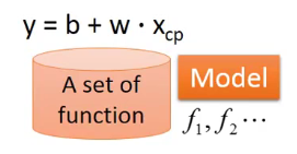
Linear model:
y
=
b
+
∑
w
i
x
i
y=b+ \sum{}^{}w_ix_i
y=b+∑wixi
x
i
x_i
xi:an attribute of input
x
x
x (feature)
w
i
w_i
wi:weight
b
b
b:bias
Step 2:Goodness of Function
Source:https://www.openintro.org/stat/data/?data=pokemon
Training Data:10 pokemons
(
x
1
,
y
^
1
)
、
(
x
2
,
y
^
2
)
、
.
.
.
、
(
x
10
,
y
^
10
)
(x^1,\hat y^1)、(x^2,\hat y^2)、...、(x^{10},\hat y^{10})
(x1,y^1)、(x2,y^2)、...、(x10,y^10)
定义Loss function L:
L
(
f
)
=
l
(
w
,
b
)
=
∑
n
=
1
10
(
y
^
n
−
(
b
+
w
∗
x
c
p
n
)
)
2
L(f)=l(w,b)=\sum_{n=1}^{10}(\hat y^n-(b+w*x_{cp}^n))^2
L(f)=l(w,b)=∑n=110(y^n−(b+w∗xcpn))2
Input:a function
output:how bad it is
Pick the “Best” Function
f
∗
=
arg min
f
L
(
f
)
f^*=\displaystyle \argmin_f L(f)
f∗=fargminL(f)
w
∗
,
b
∗
=
arg min
w
,
b
L
(
w
,
b
)
=
arg min
w
,
b
∑
n
=
1
10
(
y
^
n
−
(
b
+
w
∗
x
c
p
n
)
)
2
w^*,b^* =\displaystyle \argmin_{w,b} L(w,b)=\displaystyle \argmin_{w,b}\sum_{n=1}^{10}(\hat y^n-(b+w*x_{cp}^n))^2
w∗,b∗=w,bargminL(w,b)=w,bargminn=1∑10(y^n−(b+w∗xcpn))2
Step 3:Gradient Descent:
只要函数可微,可以找到最优的参数
Consider loss function
L
(
w
)
L(w)
L(w) with one parameter
w
w
w:
w
∗
=
arg min
w
L
(
w
)
w^*=\displaystyle \argmin_wL(w)
w∗=wargminL(w)
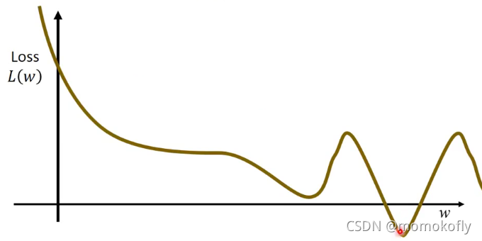
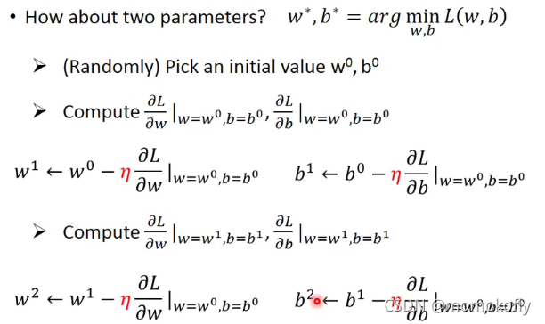
- (Randomly) Pick an initial value w 0 w^0 w0
- compute
d
L
d
w
∣
w
=
w
0
\frac{dL}{dw}|_{w=w^0}
dwdL∣w=w0,
w
1
=
w
0
−
k
d
L
d
w
∣
w
=
w
0
w^1=w^0-k\frac{dL}{dw}|_{w=w^0}
w1=w0−kdwdL∣w=w0
k k k:learning rate - compute
d
L
d
w
∣
w
=
w
1
\frac{dL}{dw}|_{w=w^1}
dwdL∣w=w1,
w
2
=
w
1
−
k
d
L
d
w
∣
w
=
w
1
w^2=w^1-k\frac{dL}{dw}|_{w=w^1}
w2=w1−kdwdL∣w=w1
…Many iteration
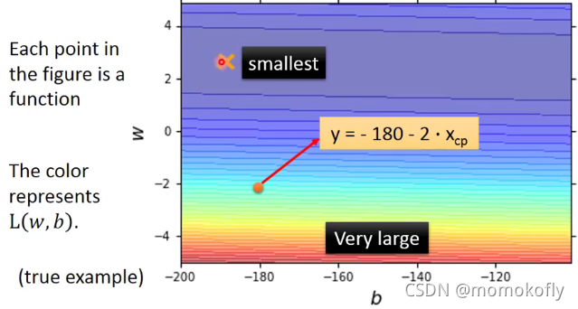
以上是对于一个参数,对于两个参数类似
下图中越偏蓝色Loss越小
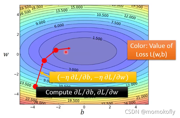
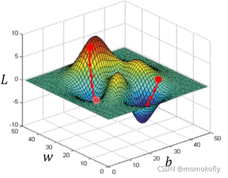
In linear regression,the loss function L is convex (no local optimal) - Formulation
L
L
L对
w
w
w和
b
b
b的偏微分值

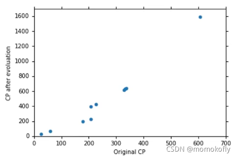
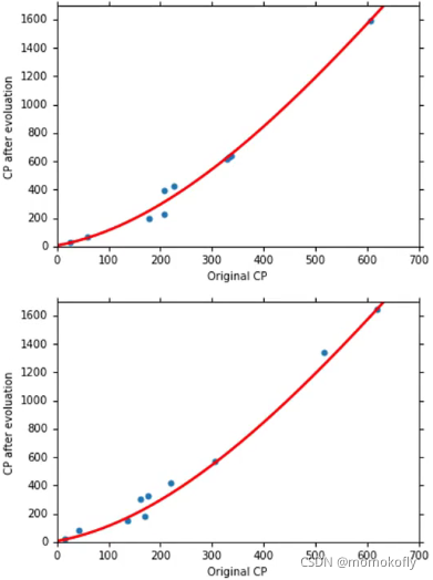
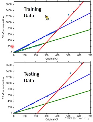
对10只pokemon进行线性回归
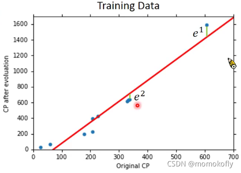
Average Error on Training Data= ∑ n = 1 10 e n \displaystyle \sum_{n=1}^{10}e_n n=1∑10en
但我们关心的是:What is the error on new data(testing data)?
testing data的误差平均值大于training data的平均误差,可能这个模型不太符合
Select another model: y = b + w 1 ∗ x c p + w 2 ∗ ( x c p ) 2 y=b+w_1*x_{cp}+w_2*(x_{cp})^2 y=b+w1∗xcp+w2∗(xcp)2
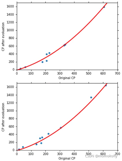
y = b + w 1 ∗ x c p + w 2 ∗ ( x c p ) 2 + w 3 ∗ ( x c p ) 3 y=b+w_1*x_{cp}+w_2*(x_{cp})^2+w_3*(x_{cp})^3 y=b+w1∗xcp+w2∗(xcp)2+w3∗(xcp)3
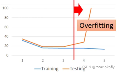
Overfitting:A more complex model does not always lead to better performance on testing data
What are the hidden factors?考虑物种区别
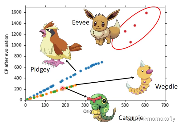
Back to step 1:Redesign the model
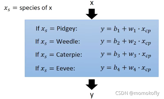
要写成线性模型,引入示性函数,如:
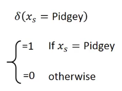
还可以考虑更加复杂的模型…但很可能发生overfitting
Back to step 2:Regularization
y
=
b
+
∑
w
i
x
i
y=b+\sum w_ix_i
y=b+∑wixi
L
=
∑
n
(
y
^
n
−
(
b
+
∑
w
i
x
i
)
)
2
+
k
∑
(
w
i
)
2
L=\displaystyle \sum_n(\hat y^n-(b+\sum w _ix_i))^2+k\sum(w_i)^2
L=n∑(y^n−(b+∑wixi))2+k∑(wi)2
The functions with smaller
w
i
w_i
wi are better
回归demo
x_data = [338,333,328,207,226,25,179,60,208,606]
y_data = [640,633,619,393,428,27,193,66,226,1591]
#ydata = b + w * xdata
b=-120 #initial b
w=-4 #initial w
lr=0.0000001 #learning rate
iteration = 100000
#Store initial values for plotting
b_history = [b]
w_history = [w]

for i in range(iteration):
	b_grad = 0.0
	w_grad = 0.0
	for n in range(len(x_data)):
		b_grad = b_grad-2.0*(y_data[n]-b-w*x_data[n]*1.0)
		w_grad = w_grad-2.0*(y_data[n]-b-w*x_data[n])*x_data[n]
	b=b-lr*b_grad
	w=w-lr*w_grad

plt.contourf(x,y,z,50,alpha = 0.5,cmap=plt.get_cmap('jet'))
plt.plot([-188.4],[2.67],'x',ms=12,markeredgewidth=3,color='orange')
plt.plot(b_history,w_history,'o-',ms=3,lw=1.5,color='black')
plt.xlim=(-200,200)
plt.ylim=(-5,5)
plt.xlabel(r'$b$',fontsize=16)
plt.ylabel(r'$w$',fontsize=16)
plt.show()
参考:https://www.bilibili.com/video/BV1Ht411g7Ef?p=3


 被折叠的 条评论
为什么被折叠?
被折叠的 条评论
为什么被折叠?
 到【灌水乐园】发言


