共享单车数据分析

共享单车数据分析

一、数据分析

1.数据特征

总共15个特征：

特征名	含义	数据形式	单位
Trip duration	骑行持续时间	23	秒
start time	骑行起始日期	2014/1/1 0:00:06	年月日
stop time	骑行终止日期	2014/1/1 0:00:12	年月日
start station id	起始站ID	2009
start station name	终止站名称	Catherine St & Monroe St
start station latitude	起始站纬度	40.71117444
start station longitude	起始站经度	-73.99682619
end station id	终止站ID	259
end station name	终止站名称	Elizabeth St & Hester St
end station latitude	终止站纬度	40.71729
end station longitude	终止站经度	-73.996375
bike id	单车ID	16379
user type	用户类型	Subscriber或Customer
birth year	用户生日	1989，单位：年
gender	性别	0或1或2

注：性别（0=未知; 1 =男性; 2 =女性）

2.数据预处理

（1）数据文件读取

首先在本地创建一个文件夹dataSet，将12 个.csv数据集文件存入该文件夹。然后输入Python的文件操作模块glob，将dataSet文件夹下所有.csv文件读取到filename中，读取文件后返回的filename为列表List格式，然后通过列表排序函数.sort()，对文件名数字排序后再打印出来。

# 获取文件名
import glob
filenames = glob.glob('dataSet/*.csv')
filenames.sort()
print(filenames)

打印输出文件名列表：

['dataSet\\2014-01 - Citi Bike trip data.csv', 'dataSet\\2014-02 - Citi Bike trip data.csv', 'dataSet\\2014-03 - Citi Bike trip data.csv', 'data
Set\\2014-04 - Citi Bike trip data.csv', 'dataSet\\2014-05 - Citi Bike trip data.csv', 'dataSet\\2014-06 - Citi Bike trip data.csv', 'dataSet\\2014-07 - Citi Bike trip data.csv', 'dataSet\\2014-08 - Citi Bike trip data.csv', 'dataSet\\2014-09 - Citi Bike trip data.csv', 'dataSet\\2014-10 - Citi Bike trip data.csv', 'dataSet\\2014-11 - Citi Bike trip data.csv', 'dataSet\\2014-12 - Citi Bike trip data.csv']

（2）合并数据文件

输入pandas模块，利用循环，逐个通过函数pd.read_csv(file)读取12个数据文件flie，然后使用函数dfs.append(pd.read_csv(file))，将12个数据文件合并为一个列表dfs，该列表含有12个元素，每个元素为一个月的数据。

import pandas as pd
# 循环读取文件数据
dfs = []
for file in filenames:
    print('Reading ' + file)
    dfs.append(pd.read_csv(file))

打印输出拼接进程：

Reading dataSet\2014-01 - Citi Bike trip data.csv
Reading dataSet\2014-02 - Citi Bike trip data.csv
Reading dataSet\2014-03 - Citi Bike trip data.csv
Reading dataSet\2014-04 - Citi Bike trip data.csv
Reading dataSet\2014-05 - Citi Bike trip data.csv
Reading dataSet\2014-06 - Citi Bike trip data.csv
Reading dataSet\2014-07 - Citi Bike trip data.csv
Reading dataSet\2014-08 - Citi Bike trip data.csv
Reading dataSet\2014-09 - Citi Bike trip data.csv
Reading dataSet\2014-10 - Citi Bike trip data.csv
Reading dataSet\2014-11 - Citi Bike trip data.csv
Reading dataSet\2014-12 - Citi Bike trip data.csv

--------------------------------------------------------------注释分割线--------------------------------------------------------------
注：
通过pd.read_csv(file)函数读取的文件，会被转化为DataFrame文件，即表格型的数据，所以dfs中的12个元素均为DataFrame文件格式。
--------------------------------------------------------------注释分割线--------------------------------------------------------------

（3）数据格式转换

在检查数据格式的时候发现9月份以后所有数据的sarttime和stoptime日期格式与其他月份的格式不同，需要进行转换。
首先检查一下8月和9月的数据格式，输出前2行查看：

dfs[7].head(2) # 检查8月份的数据

输出：

dfs[8].head(2) #检查9月的数据

输出：

dfs[9].head(2) #检查10月的数据

输出：

很明显，8月和9月份及以后的数据的sarttime和stoptime日期格式统一，因此对数据的日期格式进行统一转化为日期格式。利用pandas库的pd.to_datetime()函数。

print('Converting month:')
for month in range(12):
    if month < 8:
        print('... ' + str(month + 1))
        dfs[month]['starttime'] = pd.to_datetime(dfs[month]['starttime'])
        dfs[month]['stoptime'] = pd.to_datetime(dfs[month]['stoptime'])
    else:
        print('... ' + str(month + 1))
        dfs[month]['starttime'] = pd.to_datetime(dfs[month]['starttime'],
                                                 format = '%m/%d/%Y %H:%M:%S')
        dfs[month]['stoptime'] = pd.to_datetime(dfs[month]['stoptime'],
                                                format = '%m/%d/%Y %H:%M:%S')

输出转化过程：

Converting month:
... 1
... 2
... 3
... 4
... 5
... 6
... 7
... 8
... 9
... 10
... 11
... 12

--------------------------------------------------------------注释分割线--------------------------------------------------------------
注：
在上述转化中，为什么将8月份以前的正确的日期也转化为datetime呢？因为在DataFrame中，日期有专门的格式，为datetime。而我们原始数据中的日期，虽然字面上和日期格式相同，但Python并不能识别出来是日期格式（人和机器的区别在此），我们通过代码查看一下两种日期的格式：

#打印出未处理的9月份starttime前两行的时间
dfs[9]['starttime'].head(2)

#打印出经过转化的8月份starttime前两行的时间
dfs[7]['starttime'].head(2)

如上两图所示，日期未转化前类型为：dtype:object，经过转化的日期格式为：dtype: datetime。这个object格式一般是python用来记录可变化的兑现的格式。这个格式python并不能认出是时间格式，尽管我们一眼就能看出。
--------------------------------------------------------------注释分割线--------------------------------------------------------------

（4）拼接数据

前面通过dfs.append(pd.read_csv(file))将所有的数据都放在了dfs列表中，其有12个DataFrame元素，现在将12个DataFrame数据拼接为一个数据表df。

df = pd.concat(dfs)

查看该数据表的大小：

df.shape

输出：

(8081216, 15)

即总共有808万次骑行数据，15个特征。

（5）存储数据

存储处理后的全年数据，利用pandas的to_pickle（）函数，将数据保存在dataSet目录下的citibike_2014.pkl文件。

df.to_pickle('dataSet/citibike_2014.pkl')

--------------------------------------------------------------注释分割线--------------------------------------------------------------
注：
1.在read_csv等操作中，路径中都可以以’ \ ’符号隔开。
2.to_pickle等写入操作时，所有路径中的’ \ ‘都需要改写成’ / ’才能正常使用。
--------------------------------------------------------------注释分割线--------------------------------------------------------------

3.数据分析

（1）导入数据及相关库

第一步，导入相关库：

import numpy as np
import pandas as pd
import matplotlib as mpl
import matplotlib.pyplot as plt
plt.style.use('ggplot')  #画图风格，可以不使用
%matplotlib inline  

--------------------------------------------------------------注释分割线--------------------------------------------------------------
注：

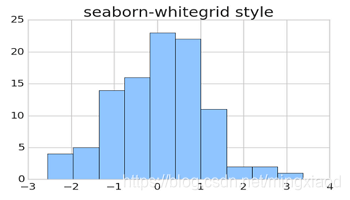
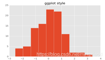
1. 画图风格，可以不使用，也可以使用其他格式，如下图为plt.style.use('seaborn-whitegrid')格式与plt.style.use('ggplot')格式的对比图。每种格式的字体、背景、画布大小都不同。
   
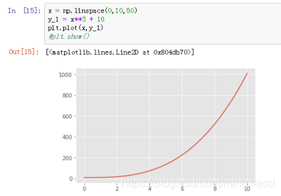
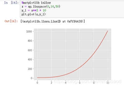
2. %matplotlib inline代码意思指在代码下方画图，一般在使用jupyter notebook 的时候才会经常用到它，在pycharm等平台中直接注释掉，否则会报错。当然在jupyter notebook中也可以不使用这条代码，直接用plt.show()即可显示图像。对比如下：很明显使用 %matplotlib inline方便很多，只需要在代码开始调用一下即可，而使用plt.show()在每次画图时都要调用一遍。
   

--------------------------------------------------------------注释分割线--------------------------------------------------------------

第二步，读取数据并测试导入数据需要的时间：

file_name = 'dataSet/citibike_2014.pkl'
%time df = pd.read_pickle(file_name)

输出：Wall time: 18.4 s #导入数据用时18.4秒
--------------------------------------------------------------注释分割线--------------------------------------------------------------
注：
当需要检测某条代码运行时间时，均可采用%time+代码的格式打印出代码的执行时间。如上述代码：%time df = pd.read_pickle(file_name)。
--------------------------------------------------------------注释分割线--------------------------------------------------------------
第三步，查看数据大小和特征格式
数据大小：

df.shape

输出：(8081216, 15)，即总共有808万次骑行数据，15个特征。

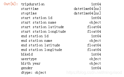
数据特征格式：

df.dtypes

输出：

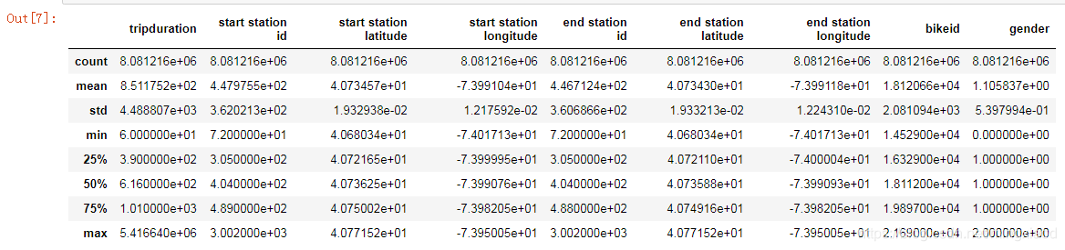
（2）数据汇总

利用pandas的describe函数（统计计数函数），可以快速的求出一些算术运算指标：

# 数值变量汇总
df.describe()

输出：

--------------------------------------------------------------注释分割线--------------------------------------------------------------

注：
count、mean、std、min、25%、50%、75%、max等代表数据集的计数，平均值，标准差，最小值，百分位数，最大值。
--------------------------------------------------------------注释分割线--------------------------------------------------------------

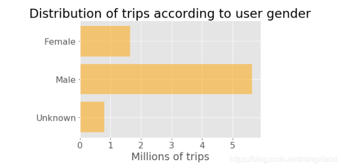
（3）用户性别的骑行分布

首先利用pandas的分组函数.groupby()，对性别的三种情况进行计数统计：

# Prepare data
genders = ['Unknown', 'Male', 'Female']
y_pos = [0, 1, 2]  #0=未知; 1 =男性; 2 =女性
trip_counts = df.groupby('gender')['gender'].count()  #根据gender分组，并根据gender类型进行计数
print(trip_counts)  #输出计数结果

如下为分组函数的统计结果：即根据性别的三种情况，统计出每一种的总数。

最后利用Matplotlib绘图：

# Plot
plt.rcParams.update({'font.size': 16})   #设置画图字体大小
plt.barh(y_pos, trip_counts / 1000000, align = 'center', alpha = 0.5, color = 'orange')  #绘制横向条形图
plt.yticks(y_pos, genders)  #设置y轴的刻度和刻标
plt.xlabel('Millions of trips') #设置x轴的刻标
plt.title('Distribution of trips according to user gender') #设置标题
plt.show()  #可使用，也可以不使用

--------------------------------------------------------------注释分割线--------------------------------------------------------------

注：
pandas中的df.groupby(‘xx’)函数指按照特征xx进行分组，如：将一个数据集按特征A进行分组, 效果是这样：

--------------------------------------------------------------注释分割线--------------------------------------------------------------

（4）用户骑行持续时间的分布

我们从上面的综述统计数据中了解到，平均行程持续时间为851秒（约14分钟），标准偏差较大（4489秒或75分钟）。 让我们更详细地看一下分布。

# 收集所有骑行持续时间大于1小时的数据
duration_mins = df.loc[(df.tripduration / 60 < 60)][['tripduration']] # 通过定位函数找到满足条件的数据，并返回骑行时长
duration_mins = duration_mins / 60 # In minutes #将骑行时长化为分钟min

# 绘制骑行时长分布图
plt.rcParams.update({'font.size': 16}) # 设置绘图字体大小
duration_mins.hist(figsize = (8,5), bins = 15, alpha = 0.5, color = 'orange') # 设置柱状图大小、柱数、透明度和颜色
plt.tick_params(axis = 'both', which = 'major', labelsize = 18) # 设置坐标参数
plt.title('Distribution of trip durations\n') # 设置图像标题
plt.xlabel('Duration (min.)') # 设置x轴标签
plt.ylabel('Trip counts') # 设置y轴标签

输出：

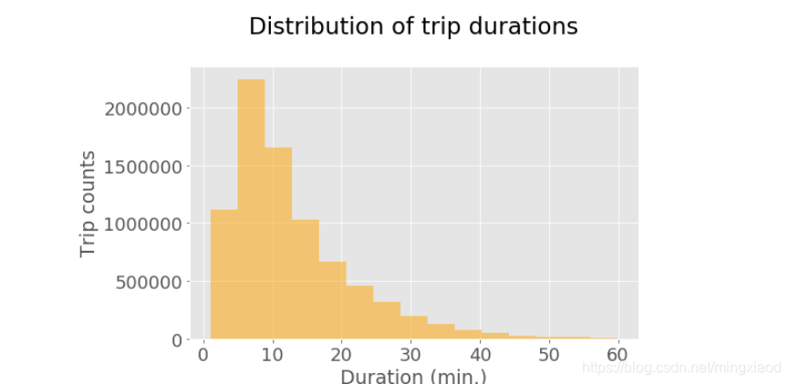
柱状图显示大多数行程都相当短。随着持续时间的增加，出行次数越来越少，长距离出行并不频繁。

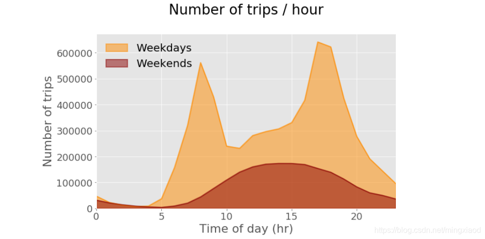
（5）单车一天内出行时刻的分布

统计出工作日和休息日每小时的行程计数

df_sub = df.loc[:, ['tripduration', 'starttime']] # 仅筛选出骑行时长和起始日期两个特征，此时数据表为多行2列
df_sub.index = df_sub['starttime'] # 将起始日期设置为DataFrame的索引
weekdays = df_sub[df_sub.index.weekday < 5] # 筛选出工作日的数据
weekends = df_sub[df_sub.index.weekday > 4] # 筛选出休息日的数据
weekdays_countsPerHr = weekdays.groupby(weekdays.index.hour).size() # 将工作日日期索引分组为小时，即得到24小时，每小时骑行的次数
weekends_countsPerHr = weekends.groupby(weekends.index.hour).size()# 将休息日日期索引分组为小时，即得到24小时，每小时骑行的次数

绘制工作日和休息日每小时骑行的次数图。

plt.rcParams.update({'font.size': 18, 'legend.fontsize': 20}) # 设置绘图字体和图例大小
weekdays_countsPerHr.plot(kind = 'area', stacked = False, figsize = (10, 6), color = 'darkorange',linewidth = 2, label='Weekdays')

weekends_countsPerHr.plot(kind = 'area', stacked = False, color = 'darkred',linewidth = 2, label='Weekends')

plt.tick_params(axis = 'both', which = 'major', labelsize = 18)
ax = plt.gca() 
plt.title('Number of trips / hour\n')
plt.xlabel('Time of day (hr)')
plt.ylabel('Number of trips')
legend = ax.legend(loc='upper left', frameon = False)

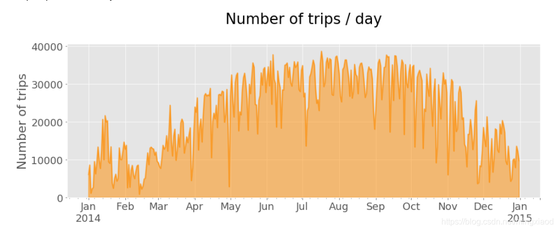
（6）单车一年内出行天的分布

df.index = df['starttime'] # 将起始日期设置为DataFrame的索引
countsPerDay = df.starttime.resample('D', how = ['count']) # 根据天数将数据表df重采样，并计数

countsPerDay.plot(kind = 'area', stacked = False, figsize = (15, 5), color = 'darkorange', linewidth = 2, legend = False)
plt.tick_params(axis = 'both', which = 'major', labelsize = 18)
#ax = plt.gca()
plt.title('Number of trips / day\n')
plt.xlabel('')
plt.ylabel('Number of trips')

输出：一年内，每天骑行次数的分布。

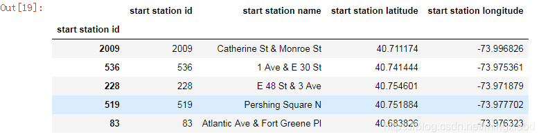
（7）起始站行程计数和租赁时间分布

仅获取起始站ID、名称和坐标，删除重复项，并添加包含每个站的行程计数和平均持续时间。

start_station = df.iloc[:,[3, 4, 5, 6]] # 即仅获取start station id、start station name、start station latitude、start station longitude四个特征
start_station.index = start_station['start station id'] # 将start station id设置为数据表的索引
start_station.head() #默认打印出前5行

输出：

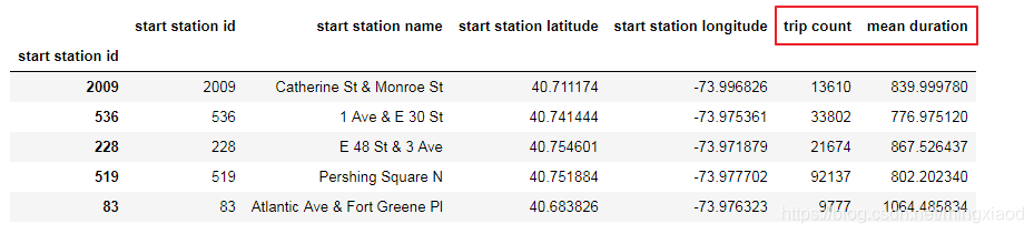
# 为每个起始站添加行程计数和平均骑行持续时间
count_start_station = df.groupby('start station id')['start station id'].count() # 根据start station id进行分组，然后通过start station id进行计数
mean_start_station = df.groupby('start station id')['tripduration'].mean() # 根据start station id进行分组，然后根据tripduration求出平均骑行持续时间
start_station['trip count'] = count_start_station # 将count_start_station数据添加到数据表start_station的列trip count
start_station['mean duration'] = mean_start_station# 将mean_start_station数据添加到数据表start_station的列mean duration
start_station.head() # 默认打印出前5行进行查看

输出：（红色部分即为添加的两列数据）

start_station = start_station.drop_duplicates() #去除重复行的数据，默认保留第一次出现的重复值
start_station.shape #输出去重之后的大小

输出：(345, 4)

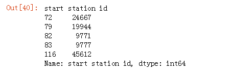
count_start_station.head() #默认输出前5行

输出：

start_station[start_station['mean duration'] > 1400] #筛选出平均骑行持续时间大于1400的起始站。

start_station['mean duration'].min() #找出平均骑行持续时间最少的起始站平均骑行时间

输出：575.1850834350835

# 制作色阶图
plt.rcParams.update({'font.size': 14})
fig = plt.figure(figsize = (.5, 30))
ax1 = fig.add_axes([0.05, 0.80, 0.9, 0.15])

# 设置与数据相对应的颜色映射和规范 
cmap = mpl.cm.YlOrRd
# 根据起始站行程次数大小绘制色阶图
norm = mpl.colors.Normalize(start_station['trip count'].min(), start_station['trip count'].max())

cb1 = mpl.colorbar.ColorbarBase(ax1, cmap = cmap, norm = norm, orientation = 'vertical')
cb1.set_label('Trip counts')

from pylab import *
savefig('color_scale_start_station.png', bbox_inches = 'tight')

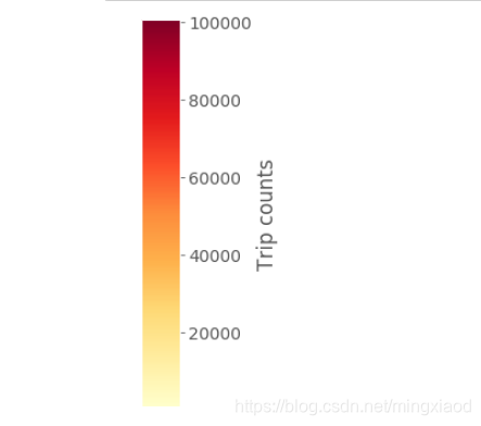
start_station['trip count'].max()

输出最大的起始站行程次数：100498

start_station['trip count'].min()

输出最小的起始站行程次数：843

start_station['mean duration'].max() / 60

输出最大的起始站平均骑行时间：64.6327552318187，单位：分钟。

start_station['mean duration'].min() / 60

输出最小的起始站平均骑行时间：9.586418057251391，单位：分钟。

二、机器学习算法

1.创建训练数据

第一步，生产训练数据。

    df[:2]
    # 删去没用信息
    new_df = df.drop(["start station name","end station name","usertype","birth year","end station latitude","end station longitude"],axis=1) # 删除一部分特征
    # del df

new_df[:10] # 打印出前10行查看

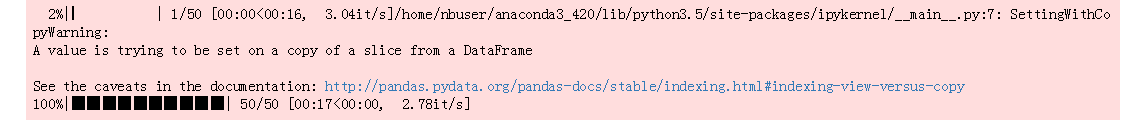
import time
from tqdm import tqdm # 导入显示进度条的模块tqdm
i = 0
times = list()
for data in new_df["starttime"]:
    data = time.strptime(str(data), "%Y-%m-%d %H:%M:%S")# 将data转化为time指定格式
    times.append(time.mktime(data))# 将数据表的startime数据格式转化为秒数
    i += 1
new_df["starttime"] = times

输出：

# 随机抽取部分用于机器学习回归
tree_df = new_df.sample(frac=0.001)
print(np.shape(new_df),np.shape(tree_df))
x = np.array(tree_df.drop(["tripduration", "stoptime"],axis=1))
y = np.array(tree_df["end station id"])

输出：(8081216, 9) (8081, 9)

第二步，创建训练数据Label标签字典
将y值转化为字典形式，并进行编码，如{地点ID：Label ID}，进而生产标签。

from sklearn.preprocessing import LabelEncoder # 导入sklearn标签编码模块
label_encoder = LabelEncoder()
label = label_encoder.fit_transform(y)# 将y值转化为字典形式，返回y标签的编码，相同数据，编码相同

label_dic = {}
for i,in_y in enumerate(list(set(label))):# 首先标签编码用set去重，然后利用enumerate同时获得索引和值
    label_dic[list(set(y))[i]] = in_y #根据编码和索引创建标签字典label_dic，即字典键为地点ID，字典值为编码

2.KNN分类器

from sklearn.neighbors import KNeighborsClassifier
from sklearn.model_selection import GridSearchCV
from sklearn.model_selection import train_test_split

X_train, X_test, y_train, y_test = train_test_split(x, label, random_state=0)
knn = KNeighborsClassifier()
knn.fit(X_train, y_train)

print("Train Num : ",len(y_train),"Test Num : ",len(y_test))

输出：Train Num : 6060 Test Num : 2021

knn.score(X_test,y_test) #计算准确率

输出：0.0054428500742206825

# 抽样检查
test_data = X_test[:20]
Linear.predict(test_data)

输出：

# 标签
y_test[:20]

输出：

3.随机森林

from sklearn.ensemble import RandomForestClassifier

cf=RandomForestClassifier()

y_RF_cf = cf.fit(X_train, y_train)

y_RF_cf.score(X_test,y_test) # 计算分类器的准确率

输出：0.3290450272142504

# 抽样检查
test_data = X_test[:20]
y_RF_cf.predict(test_data)

输出：

# 标签
y_test[:20]

输出：

三、深度学习算法

1.循环神经网络

（1）分割训练集与验证集

x = np.array(new_df.drop(["tripduration", "stoptime"],axis=1))# 去掉tripduratio和stoptime两个特征
y = np.array(new_df["end station id"]) #将end station id设置为y值

label_encoder = LabelEncoder()
label = label_encoder.fit_transform(y)# 将y值转化为字典形式，返回y标签的编码，相同数据，编码相同

label_dic = {}
for i,in_y in enumerate(list(set(label))): # 首先标签编码用set去重，然后利用enumerate同时获得索引和值
    label_dic[list(set(y))[i]] = in_y #根据编码和索引创建标签字典label_dic
    
X_train, X_test, y_train, y_test = train_test_split(x, y, random_state=0)#划分训练子集和测试子集

（2）导入包和定义层

导入需要用到的包

from keras import Sequential
from keras.preprocessing.sequence import pad_sequences
from sklearn.model_selection import train_test_split
from keras.models import Sequential,Model
from keras.layers import LSTM, Dense, Bidirectional, Input,Dropout,BatchNormalization, CuDNNGRU, CuDNNLSTM,Add,Conv1D,Dropout
from keras import backend as K
from keras.engine.topology import Layer
from keras import initializers, regularizers,constraints

定义attention层的

# 参考论文 《Attention is all you need》
class Attention(Layer):
    def __init__(self, step_dim,
                 W_regularizer=None, b_regularizer=None,
                 W_constraint=None, b_constraint=None,
                 bias=True, **kwargs):
        self.supports_masking = True
        self.init = initializers.get('glorot_uniform')

        self.W_regularizer = regularizers.get(W_regularizer)
        self.b_regularizer = regularizers.get(b_regularizer)

        self.W_constraint = constraints.get(W_constraint)
        self.b_constraint = constraints.get(b_constraint)

        self.bias = bias
        self.step_dim = step_dim
        self.features_dim = 0
        super(Attention, self).__init__(**kwargs)

    def build(self, input_shape):
        assert len(input_shape) == 3

        self.W = self.add_weight((input_shape[-1],),
                                 initializer=self.init,
                                 name='{}_W'.format(self.name),
                                 regularizer=self.W_regularizer,
                                 constraint=self.W_constraint)
        self.features_dim = input_shape[-1]

        if self.bias:
            self.b = self.add_weight((input_shape[1],),
                                     initializer='zero',
                                     name='{}_b'.format(self.name),
                                     regularizer=self.b_regularizer,
                                     constraint=self.b_constraint)
        else:
            self.b = None

        self.built = True

    def compute_mask(self, input, input_mask=None):
        return None

    def call(self, x, mask=None):
        features_dim = self.features_dim
        step_dim = self.step_dim

        eij = K.reshape(K.dot(K.reshape(x, (-1, features_dim)),
                        K.reshape(self.W, (features_dim, 1))), (-1, step_dim))

        if self.bias:
            eij += self.b

        eij = K.tanh(eij)

        a = K.exp(eij)

        if mask is not None:
            a *= K.cast(mask, K.floatx())

        a /= K.cast(K.sum(a, axis=1, keepdims=True) + K.epsilon(), K.floatx())

        a = K.expand_dims(a)
        weighted_input = x * a
        return K.sum(weighted_input, axis=1)

    def compute_output_shape(self, input_shape):
        return input_shape[0],  self.features_dim

（3）包含Attention机制的LSTM

LSTM全称：long short term memory，属于循环神经网络RNN。

# 建立网络流程
model = Sequential()
model.add(BatchNormalization(input_shape=(1, 7)))
model.add(Bidirectional(LSTM(16, dropout=0.4, recurrent_dropout=0.4, activation='relu', return_sequences=True)))
model.add(Bidirectional(LSTM(32, return_sequences=True)))
model.add(BatchNormalization(input_shape=(1, 32)))
model.add(Bidirectional(LSTM(64, activation='tanh', return_sequences = True)))
model.add(BatchNormalization(input_shape=(1, 64)))
model.add(Attention(64))
model.add(Dense(512,activation="relu"))
model.add(Dropout(0.3))
model.add(Dense(512,activation="relu"))
model.add(Dropout(0.3))
model.add(Dense(len(list(set(y))),activation="softmax"))
model.compile(loss='binary_crossentropy', optimizer='adam', metrics=['accuracy'])
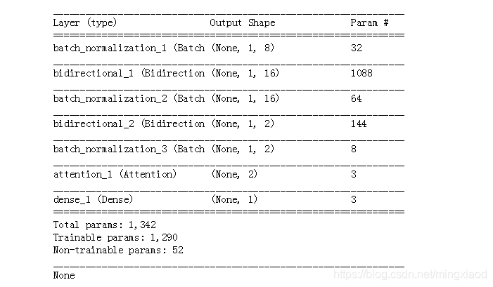
print(model.summary())

输出：

from sklearn.preprocessing import OneHotEncoder
X_train = np.reshape(X_train,[-1,1,7])
X_test = np.reshape(X_test,[-1,1,7])
one_hot = OneHotEncoder()
temp = one_hot.fit_transform(np.reshape(y_test,[-1,1])).toarray()
print(y_test)
print(temp[:10])
print(np.shape(temp))

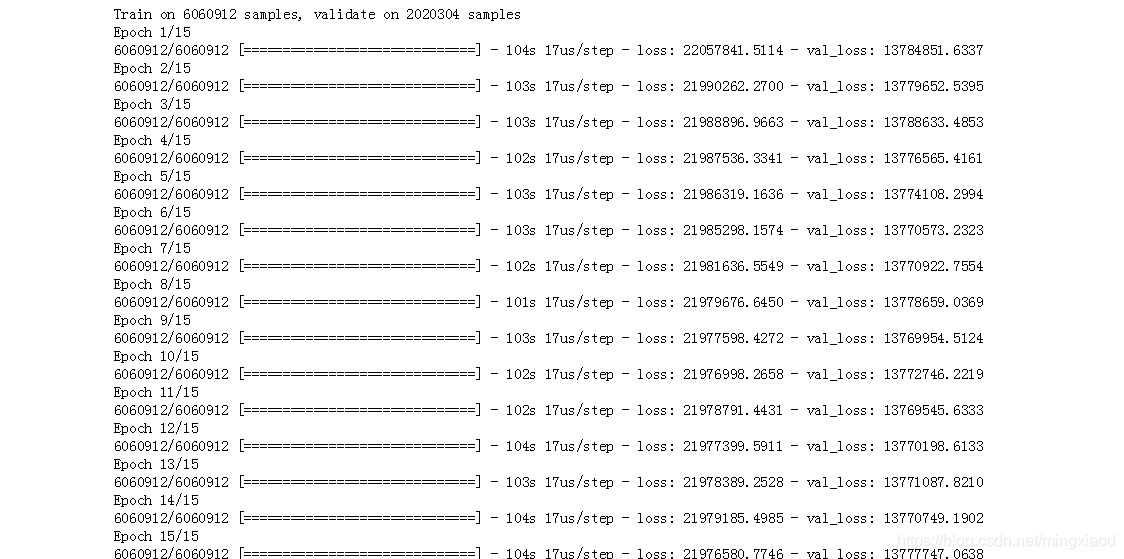
# 训练神经网络
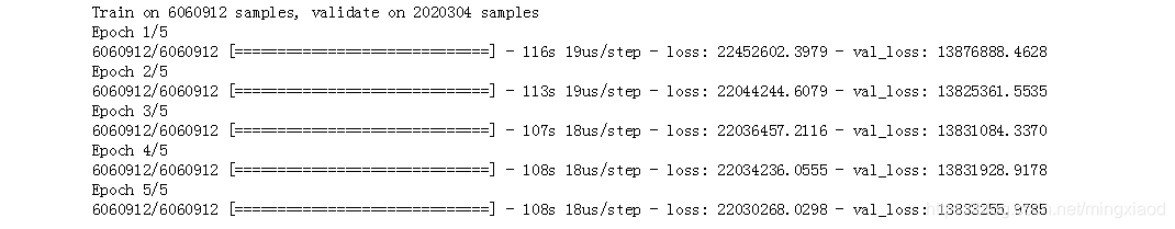
history = model.fit(X_train, y_train,batch_size=300,epochs=15,validation_data=(X_test, y_test))

输出：

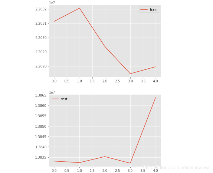
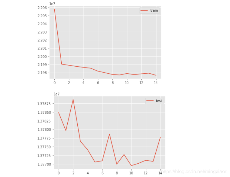
# 绘制折线图
from matplotlib import pyplot

pyplot.plot(history.history['loss'], label='train')
# pyplot.plot(history.history['val_loss'], label='test')
pyplot.legend()
pyplot.show()
# pyplot.plot(history.history['loss'], label='train')
pyplot.plot(history.history['val_loss'], label='test')
pyplot.legend()
pyplot.show()

输出：

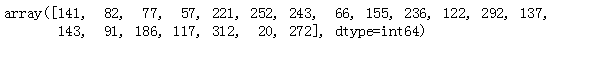
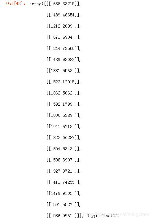
model.predict(X_test[:20])

输出：

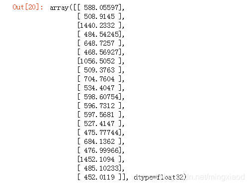
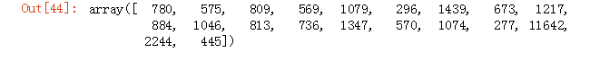
y_test[:20]

输出：

--------------------------------------------------------------注释分割线--------------------------------------------------------------

注：

1. 网络层含义
   Sequential：多个网络层的线性堆叠
   BatchNormalization：规范化层，对批次数据进行规范化
   Bidirectional:属于包装器层，Bidirectional用于双向RNN包装器
   Dense：全连接层
   model层：
   model.compile:传入损失函数binary_crossentropy（亦称作对数损失），优化器Adam，模型评估指标accuracy
   model.summary()：模型概况
2. 模型参数含义
   input_shape：输入张量的大小
   units：RNN的单元数，也是输出维度
   activation：激活函数，为预定义的激活函数名
   dropout：0~1之间的浮点数，控制输入线性变换的神经元断开比例，防止过拟合
   recurrent_dropout：0~1之间的浮点数，控制循环状态的线性变换的神经元断开比例
   return_sequences：True返回整个序列，False返回输出序列的最后一个输出
3. 模型训练参数含义
   model.fit(X_train, y_train,batch_size=300,epochs=15,validation_data=(X_test, y_test))
   X_train：输入训练数据
   y_train：输入训练标签
   batch_size：指定进行梯度下降时每个batch包含的样本数为300
   epochs：训练的轮数，训练数据将会被遍历epoch次，即15次
   validation_data：指定验证集为X_test, y_test
   --------------------------------------------------------------注释分割线--------------------------------------------------------------

（4）不包含Attention机制的LSTM

# 建立网络流程
model = Sequential()
model.add(BatchNormalization(input_shape=(1, 7)))
model.add(Bidirectional(LSTM(16, dropout=0.4, recurrent_dropout=0.4, activation='relu', return_sequences=True)))
model.add(Bidirectional(LSTM(32, return_sequences=True)))
model.add(BatchNormalization(input_shape=(1, 32)))
model.add(Bidirectional(LSTM(64, activation='tanh', return_sequences = True)))
model.add(BatchNormalization(input_shape=(1, 64)))
# model.add(Attention(1))
model.add(Dense(512,activation="relu"))
model.add(Dropout(0.3))
model.add(Dense(512,activation="relu"))
model.add(Dropout(0.3))
model.add(Dense(len(list(set(y))),activation="softmax"))
model.compile(loss='binary_crossentropy', optimizer='adam', metrics=['accuracy'])
print(model.summary())

输出：

# 训练神经网络
history = model.fit(X_train, np.reshape(y_train,[-1,1,1]),
          batch_size=300,
          epochs=15,
          validation_data=(X_test, np.reshape(y_test,[-1,1,1])))

输出：

# 绘制折线图
from matplotlib import pyplot

pyplot.plot(history.history['loss'], label='train')
# pyplot.plot(history.history['val_loss'], label='test')
pyplot.legend()
pyplot.show()
# pyplot.plot(history.history['loss'], label='train')
pyplot.plot(history.history['val_loss'], label='test')
pyplot.legend()
pyplot.show()

输出：

model.predict(X_test[:20])

输出：

y_test[:20]

输出：

2.BP神经网络

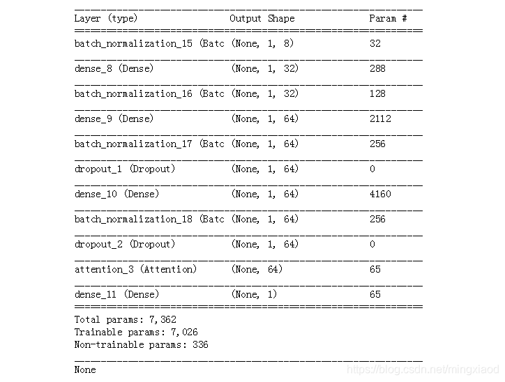
（1）包含Attention机制的BP

# 建立网络流程
model = Sequential()
model.add(BatchNormalization(input_shape=(1, 7)))
model.add(Dense(256,activation='relu'))
model.add(BatchNormalization(input_shape=(1, 256)))
model.add(Dense(500,activation='relu'))
model.add(BatchNormalization(input_shape=(1, 500)))
model.add(Dropout(0.3))
model.add(Dense(500,activation='relu'))
model.add(BatchNormalization(input_shape=(1, 500)))
model.add(Dropout(0.4))
model.add(Attention(1))
model.add(Dense(len(list(set(y))),activation="softmax"))
model.compile(loss='binary_crossentropy', optimizer='adam', metrics=['accuracy'])
print(model.summary())

输出：

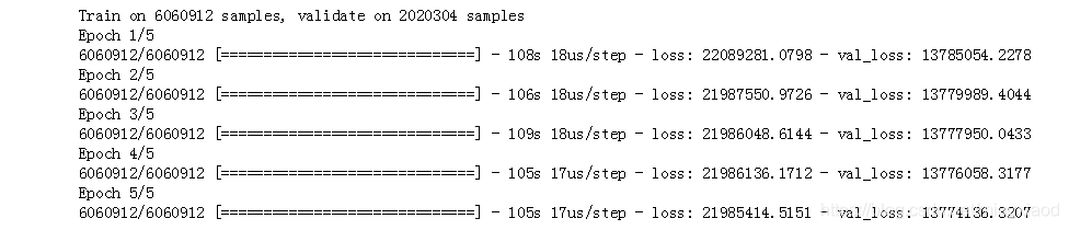
# 训练神经网络
history = model.fit(X_train, y_train,
          batch_size=300,
          epochs=15,
          validation_data=(X_test, y_test))

输出：

# 绘制折线图
from matplotlib import pyplot

pyplot.plot(history.history['loss'], label='train')
# pyplot.plot(history.history['val_loss'], label='test')
pyplot.legend()
pyplot.show()
# pyplot.plot(history.history['loss'], label='train')
pyplot.plot(history.history['val_loss'], label='test')
pyplot.legend()
pyplot.show()

输出：

model.predict(X_test[:20])

输出：

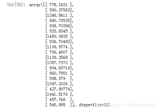
y_test[:20]

输出：

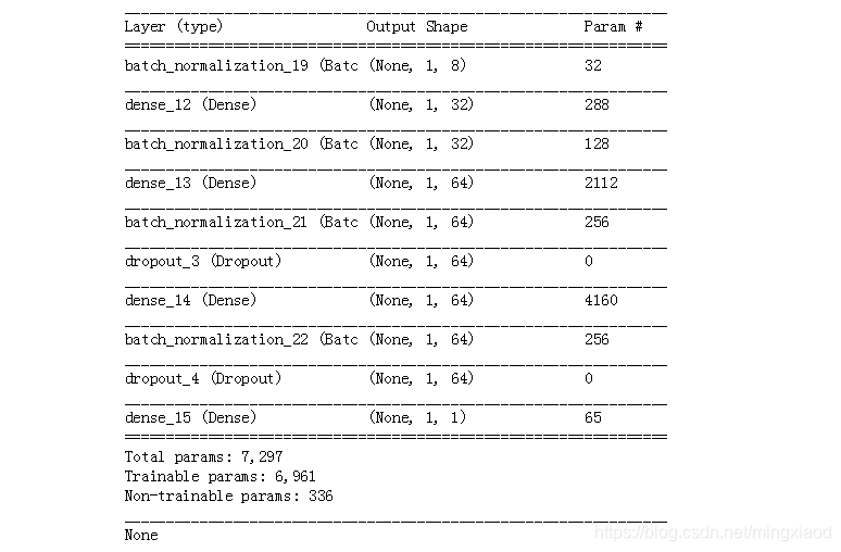
（2）不包含Attention机制的BP

# 建立网络流程
model = Sequential()
model.add(BatchNormalization(input_shape=(1, 7)))
model.add(Dense(256,activation='relu'))
model.add(BatchNormalization(input_shape=(1, 256)))
model.add(Dense(512,activation='relu'))
model.add(BatchNormalization(input_shape=(1, 512)))
model.add(Dropout(0.3))
model.add(Dense(512,activation='relu'))
model.add(BatchNormalization(input_shape=(1, 512)))
model.add(Dropout(0.4))
model.add(Dense(len(list(set(y))),activation="softmax"))
model.compile(loss='binary_crossentropy', optimizer='adam', metrics=['accuracy'])
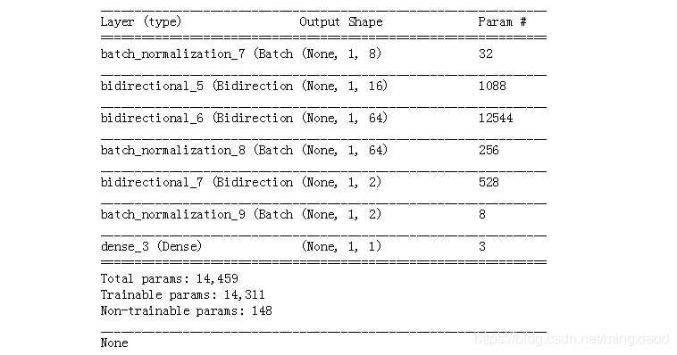
print(model.summary())

输出：

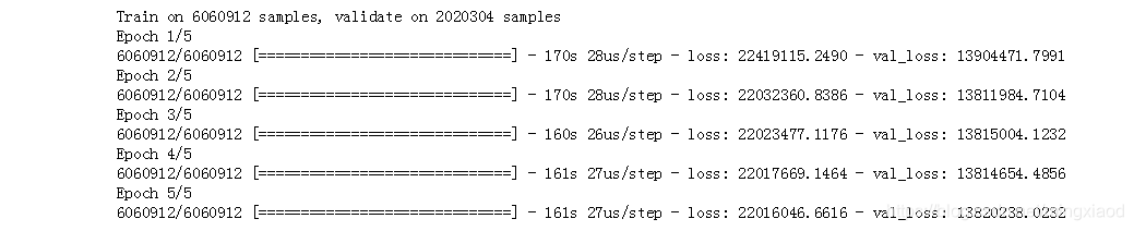
# 训练神经网络
history = model.fit(X_train, np.reshape(y_train,[-1,1,1]),
          batch_size=300,
          epochs=15,
          validation_data=(X_test, np.reshape(y_test,[-1,1,1])))

输出：

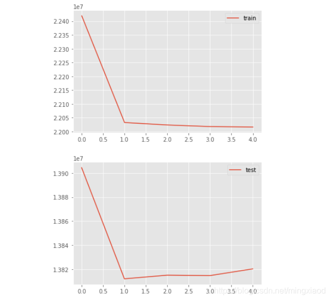
# 绘制折线图
from matplotlib import pyplot

pyplot.plot(history.history['loss'], label='train')
# pyplot.plot(history.history['val_loss'], label='test')
pyplot.legend()
pyplot.show()
# pyplot.plot(history.history['loss'], label='train')
pyplot.plot(history.history['val_loss'], label='test')
pyplot.legend()
pyplot.show()

输出：

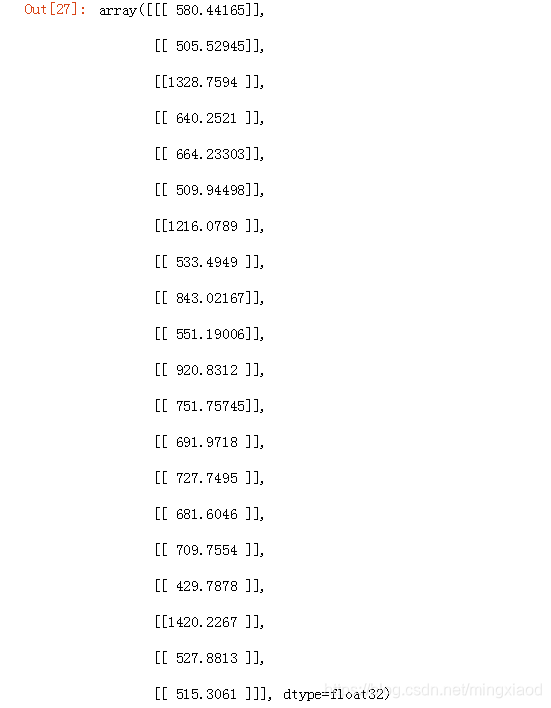
model.predict(X_test[:20])

输出：

y_test[:20]

输出：