


 RAFT是一种新的光流估计方法,抛弃了coarse-to-fine策略,采用全尺寸光流估计,利用CNN-GRU进行迭代优化,提高了准确性并减少了计算复杂度。在1080 TI GPU上实现10FPS。实验表明,RAFT在光流估计中表现出色,具有较好的泛化性能。
参考代码:RAFT
作者主页:Zachary Teed
1. 概述
导读:这篇文章提出了一种新的光流估计pipline,与之前介绍的PWC-Net类似其也包含特征抽取/correlation volume构建操作。在这篇文章中为了优化光流估计,首先在correlation volume的像素上进行邻域采样得到lookups特征(增强特征相关性,也可以理解为感受野),之后直接使用以CNN-GRU为基础的迭代优化网络,在完整尺寸上对光流估计迭代优化。这样尽管采用了迭代优化的形式,文章的迭代优化机制也比像IRR/FlowNet这类方法轻量化,运行速度也更快,其可以在1080 TI GPU上达到10FPS(输入为 1088 ∗ 436 1088*436 1088∗436)。文章的算法在诸如特征处理与融合/上采样策略上设计得细致合理,并且使用迭代优化的策略,从而使得文章算法具有较好的泛化性能。
将文章的方法与之前的一些方法作对比,可以将其中对比得到的改进点归纳如下:
- 1)抛弃了类似PWC-Net中的coarse-to-fine的光流迭代优化策略,直接生成全尺寸的光流估计,从而避免了这种优化策略带来的弊端:coarse层次的预测结果会天然增加丢失小而快速运动的目标的风险,并且训练需要的迭代次数也更多;
- 2)为了提升光流估计的准确性,一种可行的方式就是进行module的叠加优化,如FlowNet和IRR等,但是这样的操作一个是带来更多的参数量,增加运算的时间。还会使得整个网络的训练过程变得繁琐冗长;
- 3)光流的更新模块,文章使用以CNN-GRU为基础,在4D的correlation volume上对其采样得到的correlation lookups进行运算,从而得到光流信息。这样的更新模块引入了GRU网络,很好利用了迭代优化的时序特性;
将文章的方法与其它的一些光流估计方法进行比较:

2. 方法设计
2.1 整体pipline
文章的整体pipeline如下:

按照上图所示可以将整体pipeline划分为3个部分(阶段):
- 1)feature encoder进行输入图像的抽取,以及context encoder进行图像特征的抽取;
- 2)使用矩阵相乘的方式构建correlation volume,之后使用池化操作得到correlation volume pyramid;
- 3)对correlation volume在像素邻域上进行采样,之后使用以CNN-GRU为基础构建的光流迭代更新网络进行全尺寸光流估计;
文章按照网络容量的不同设计了一大一小的两个网络,后面的内容都是以大网络为基准,其网络结构为:

文章的整体流程简洁,直接在一个forawrd中完成了所有操作,其具体的步骤可以归纳为:
# core/raft.py#86
# step1:图像1/2的feature encoder特征抽取
fmap1, fmap2 = self.fnet([image1, image2])  # [N, 256, H//8, W//8]

# step2:correlation volume pyramid构建
if self.args.alternate_corr:
    corr_fn = AlternateCorrBlock(fmap1, fmap2, radius=self.args.corr_radius)
else:
    corr_fn = CorrBlock(fmap1, fmap2, radius=self.args.corr_radius)  # 输入两幅图像特征用于构造金字塔相似矩阵

# step3:图像1的context encoder特征抽取
cnet = self.cnet(image1)
net, inp = torch.split(cnet, [hdim, cdim], dim=1)  # 对输出的特征进行划分
# 一部分用于递归优化的输入,一部分用于GRU递归优化的传递变量
net = torch.tanh(net)  # [N, 256, H//8, W//8]
inp = torch.relu(inp)  # [N, 256, H//8, W//8]

# step4:以图像1经过编码之后的尺度构建两个一致的坐标网格
coords0, coords1 = self.initialize_flow(image1)  # 一个用于更新(使用每次迭代预测出来的光流),一个用于作为基准

if flow_init is not None:  # 若初始光流不为空,则用其更新初始光流
    coords1 = coords1 + flow_init

# step5:进行光流更新迭代
flow_predictions = []
for itr in range(iters):
    coords1 = coords1.detach()
    # 在坐标网格的基础上对correlation volume pyramid进行半径r=4的邻域采样
    corr = corr_fn(coords1)  # index correlation volume [N, (2*r+1)*(2*r+1)*num_levels, H//8, W//8]

    # 使用CNN-GRU计算光流偏移量与上采样系数等
    flow = coords1 - coords0
    with autocast(enabled=self.args.mixed_precision):
        net, up_mask, delta_flow = self.update_block(net, inp, corr, flow)  # 迭代之后的特征/采样权重/预测光流偏移

    # F(t+1) = F(t) + \Delta(t)
    coords1 = coords1 + delta_flow  # 更新光流

    # upsample predictions
    if up_mask is None:
        flow_up = upflow8(coords1 - coords0)  # 普通的上采样方式
    else:
        flow_up = self.upsample_flow(coords1 - coords0, up_mask)  # 使用卷积构造的上采样方式

    flow_predictions.append(flow_up)  # 保存当前迭代次数的光流优化结果
2.2 correlation volume
这里主要讲述correlation volume的构建过程,之后在其基础上进行邻域采样构建correlation lookups(用于提升光流信息的特征相关性),以及提出一种更加高效的correlation volume构建方式(减少计算复杂度)。这里的编码器特征抽取部分省略。。。(其输出的维度为: [ N , 256 , H / / 8 , H / / 8 ] [N,256,H//8,H//8] [N,256,H//8,H//8])
构建过程:
correlation volume的构建过程其实是一个矩阵相乘形式:
# core/corr.py#53
def corr(fmap1, fmap2):
    batch, dim, ht, wd = fmap1.shape
    fmap1 = fmap1.view(batch, dim, ht*wd)
    fmap2 = fmap2.view(batch, dim, ht*wd)

    corr = torch.matmul(fmap1.transpose(1,2), fmap2)  # 图像1/2的特征矩阵乘 [batch, ht*wd, ht*wd]
    corr = corr.view(batch, ht, wd, 1, ht, wd)  # [batch, ht, wd, 1, ht, wd]
    return corr  / torch.sqrt(torch.tensor(dim).float())
在此基础上使用池化操作得到correlation volume,这里使用到的层级为4(池化操作的kernel size为
{
1
,
2
,
4
,
8
}
\{1,2,4,8\}
{1,2,4,8})。也就如下图所示:

correlation lookups的构建:
这里为了增加correlation volume中每个像素对周围像素的感知能力,使用半径
r
=
4
r=4
r=4的邻域对correlation volume中每个像素进行采样,之后再组合起来。其实现可以参考:
# core/corr.py#29
def __call__(self, coords):
    r = self.radius
    coords = coords.permute(0, 2, 3, 1)  # flow的idx坐标信息permute
    batch, h1, w1, _ = coords.shape  # [batch, h1, w1, 2]

    out_pyramid = []
    for i in range(self.num_levels):
        corr = self.corr_pyramid[i]
        dx = torch.linspace(-r, r, 2*r+1)  # 构造邻域采样空间
        dy = torch.linspace(-r, r, 2*r+1)
        delta = torch.stack(torch.meshgrid(dy, dx), axis=-1).to(coords.device)

        centroid_lvl = coords.reshape(batch*h1*w1, 1, 1, 2) / 2**i  # 将光流缩放到对应的金字塔尺度上去
        delta_lvl = delta.view(1, 2*r+1, 2*r+1, 2)  # 邻域区域,邻域半径r=4
        coords_lvl = centroid_lvl + delta_lvl  # 在光流基础上加上邻域区域的偏置,[batch*h1*w1, 2*r+1, 2*r+1, 2]

		# 在邻域上对correlation volume在坐标coords_lvl引导下进行双线性采样
        corr = bilinear_sampler(corr, coords_lvl)  # [batch*h1*w1, 1, 2*r+1, 2*r+1]
        corr = corr.view(batch, h1, w1, -1)  # [batch, h1, w1, (2*r+1) * (2*r+1)]
        out_pyramid.append(corr)

    out = torch.cat(out_pyramid, dim=-1)  # [batch, h1, w1, (2*r+1) * (2*r+1) * num_levels]
    return out.permute(0, 3, 1, 2).contiguous().float()    # [batch, (2*r+1) * (2*r+1) * num_levels, h1, w1]
更加高效的correlation构建:
在之前的correlation volume构建过程中是直接在编码器输出的特征图上运算,其计算的复杂度为
O
(
N
2
)
O(N^2)
O(N2),其中
N
N
N是特征图上像素的个数(
W
/
/
8
∗
H
/
/
8
W//8*H//8
W//8∗H//8,channel=1)。之后这个保持不变,使用不同kernel size的池化操作迭代计算
M
M
M次(也就是金字塔的层级)。那么对此文章对于层级为
m
m
m处correlation volume的计算其实是可以描述为下面的形式的:
C
i
j
k
l
m
=
1
2
2
m
∑
p
2
m
∑
q
2
m
⟨
g
i
,
j
(
1
)
,
g
2
m
k
+
p
,
2
m
l
+
q
(
2
)
⟩
=
⟨
g
i
,
j
(
1
)
,
1
2
2
m
(
∑
p
2
m
∑
q
2
m
g
2
m
k
+
p
,
2
m
l
+
q
(
2
)
)
⟩
C_{ijkl}^m=\frac{1}{2^{2m}}\sum_p^{2^m}\sum_q^{2^m}\langle g_{i,j}^{(1)},g_{2^mk+p,2^ml+q}^{(2)}\rangle=\langle g_{i,j}^{(1)},\frac{1}{2^{2m}}(\sum_p^{2^m}\sum_q^{2^m}g_{2^mk+p,2^ml+q}^{(2)})\rangle
Cijklm=22m1p∑2mq∑2m⟨gi,j(1),g2mk+p,2ml+q(2)⟩=⟨gi,j(1),22m1(p∑2mq∑2mg2mk+p,2ml+q(2))⟩
也就是图像1的特征与图像2图像块avg-pooling之后的特征进行计算,进而可以减少计算复杂度,变为$O(NM)。其实现可以参考类:
#core/corr.py#63
class AlternateCorrBlock:
	...
以及目录alt_cuda_corr下的实现。
2.3 迭代更新机制
文章的光流估计是采用迭代更新的机制实现的,也就是在一个迭代序列中会生成光流序列
{
f
1
,
…
,
f
N
}
\{f_1,\dots,f_N\}
{f1,…,fN},初始情况下
f
0
=
0
f_0=0
f0=0,每次迭代之后的更新量描述为
Δ
f
\Delta f
Δf,那么其更新过程描述为:
f
k
+
1
=
f
k
+
Δ
f
f_{k+1}=f_k+\Delta f
fk+1=fk+Δf
迭代更新的初始值:
在缺省情况下文章的方法是使用0作迭代的初始光流。当然也是可以接受用一个先验光流作为输入,并在该基础上进行更新迭代,也就是文章提到的warm-start。
迭代更新的输入:
在上文中的网络结构图中可以看到输入CNN-GRU网络模块中的信息是包含3个:context encoder的输出特征/上一次光流的迭代结果/correlation volume在邻域内的采样结果。它们在网络中通过concat的形式进行特征融合,融合之后的特征记为
x
t
x_t
xt。
特征更新过程:
光流在进行估计之前会经过CNN-GRU模块,这里采用的是Separate的形式,也就是分离的大卷积核(减少参数量的同时,增大感受野)。这里循环递归的隐变量为
h
t
h_t
ht,它初始的时候使用context encoder产生。其在GRU模块中更新的过程可以描述为:
z
t
=
σ
(
C
o
n
v
3
∗
3
(
[
h
t
−
1
,
x
t
]
,
W
z
)
)
z_t=\sigma(Conv_{3*3}([h_{t-1},x_t],W_z))
zt=σ(Conv3∗3([ht−1,xt],Wz))
r
t
=
σ
(
C
o
n
v
3
∗
3
(
[
h
t
−
1
,
x
t
]
,
W
r
)
)
r_t=\sigma(Conv_{3*3}([h_{t-1},x_t],W_r))
rt=σ(Conv3∗3([ht−1,xt],Wr))
h
ˉ
t
=
t
a
n
h
(
C
o
n
v
3
∗
3
[
r
t
⊙
h
t
−
1
,
x
t
]
,
W
h
)
\bar{h}_t=tanh(Conv_{3*3}[r_t\odot h_{t-1},x_t],W_h)
hˉt=tanh(Conv3∗3[rt⊙ht−1,xt],Wh)
h
t
=
(
1
−
z
t
)
⊙
h
t
−
1
+
z
t
⊙
h
ˉ
t
h_t=(1-z_t)\odot h_{t-1}+z_t\odot \bar{h}_t
ht=(1−zt)⊙ht−1+zt⊙hˉt
光流更新量估计:
这里估计的光流其实是一个偏移量
Δ
f
\Delta f
Δf,相对坐标矩阵来讲的。最后将变换后的坐标矩阵减去之前的基准就得到了最后的光流估计。
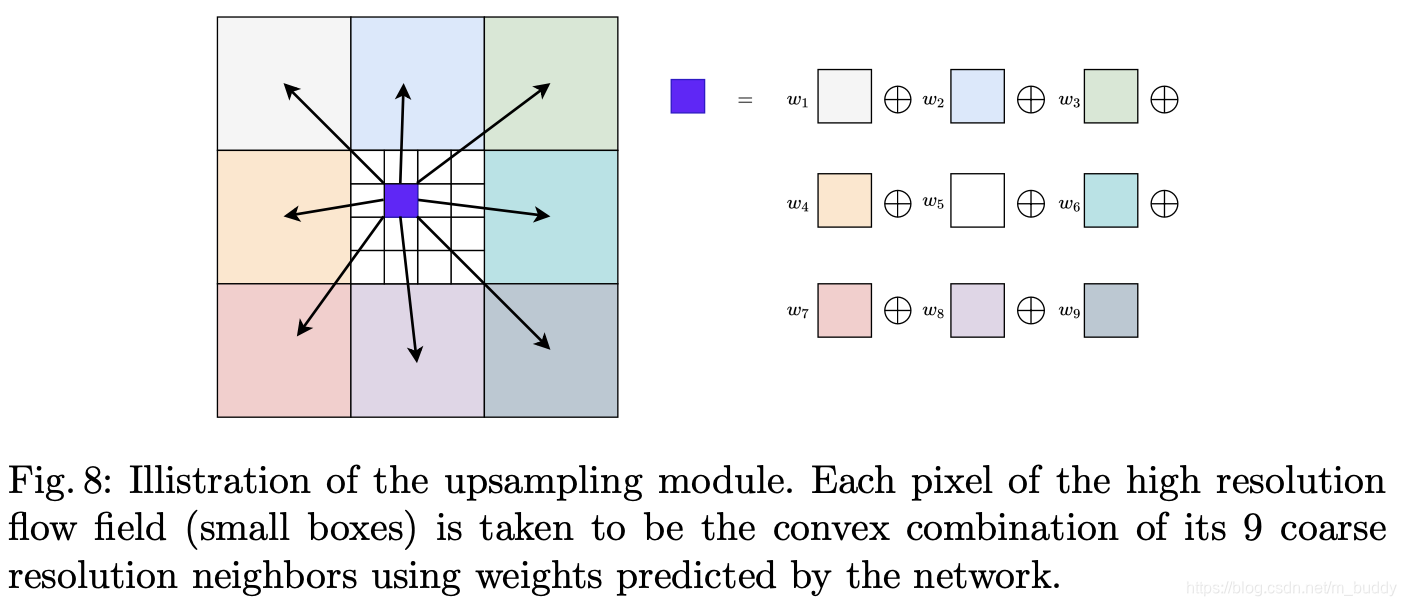
全尺寸上采样:
这里将传统的双线性采样操作替换为了基于卷积的上采样操作,也就是每个全尺寸中的每个像素是通过在stride=8的光流预测结果对应位置处采样
3
∗
3
3*3
3∗3的块,之后通过预测出来的权值进行加权组合。其采样加权的示意图如下:
其实现代码参考:
# core/raft.py#72
def upsample_flow(self, flow, mask):
    """ Upsample flow field [H/8, W/8, 2] -> [H, W, 2] using convex combination """
    N, _, H, W = flow.shape
    mask = mask.view(N, 1, 9, 8, 8, H, W)  # [N, 8*8*9, H, W]->[N, 1, 9, 8, 8, H, W]
    mask = torch.softmax(mask, dim=2)  # 当前像素与邻域像素的权值

    up_flow = F.unfold(8 * flow, [3, 3], padding=1)  # 对光流进行窗口滑块提取[N, 3*3*2, H, W](提前乘上采样系数8)
    up_flow = up_flow.view(N, 2, 9, 1, 1, H, W)  # [N, 3*3*2, H, W]->[N, 2, 9, 1, 1, H, W]

    up_flow = torch.sum(mask * up_flow, dim=2)  # 当前像素与邻域进行加权计算, [N, 2, 9, 1, 1, H, W]->[N, 2, 8, 8, H, W]
    up_flow = up_flow.permute(0, 1, 4, 2, 5, 3)  # [N, 2, 8, 8, H, W]->[N, 2, H, 8, W, 8]
    return up_flow.reshape(N, 2, 8*H, 8*W)  # 得到输入图像分辨率的光流估计
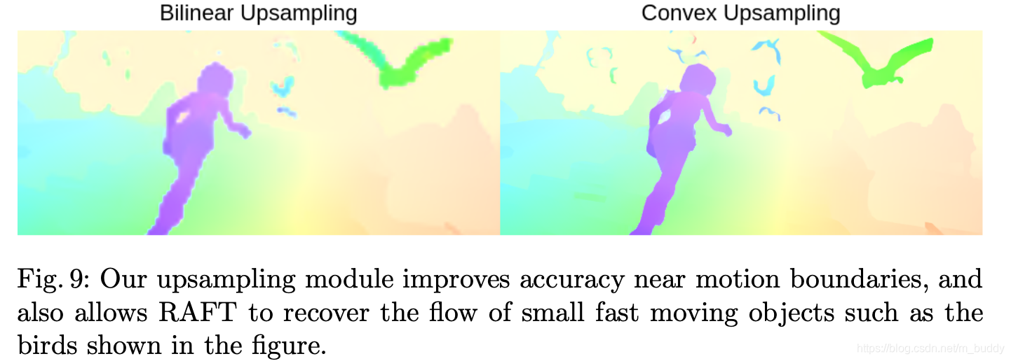
将直接双线性上采样的结果与这里提出的上采样结果进行对比如下:
2.4 损失函数
文章的方法是迭代更新的,因而会生成许多个序列的光流估计结果
{
f
1
,
…
,
f
N
}
\{f_1,\dots,f_N\}
{f1,…,fN},对此其损失函数描述为:
L
=
∑
i
=
1
N
γ
N
−
i
∣
f
g
t
−
f
i
∣
1
L=\sum_{i=1}^N\gamma^{N-i}|f_{gt}-f_i|_1
L=i=1∑NγN−i∣fgt−fi∣1
其中,
γ
=
0.8
\gamma=0.8
γ=0.8。
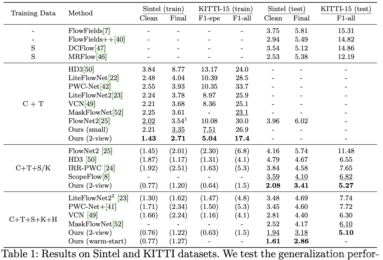
3. 实验结果
KITTI数据集上的性能比较:
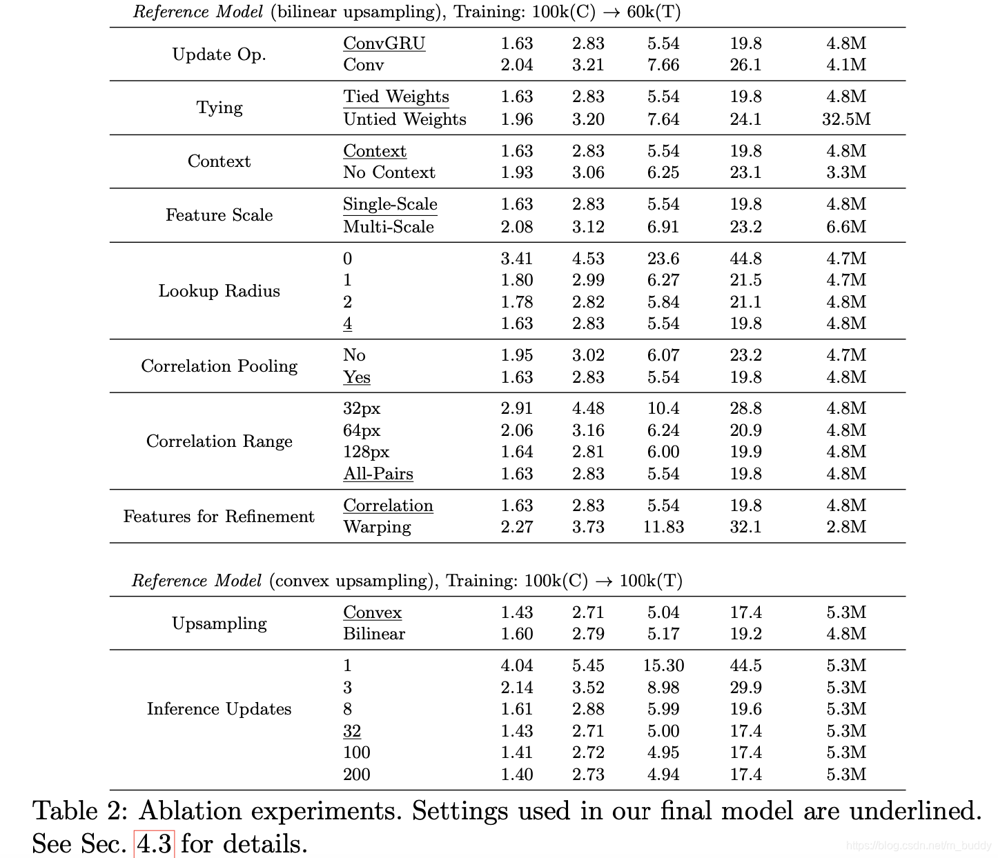
消融实验:
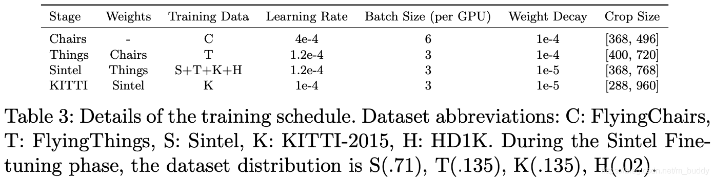
训练策略:


 6545
6545


 到【灌水乐园】发言


