离散时间信号的实现和时域基本运算（9）

实验目的

1）了解时域离散信号的特点；
2）掌握MATLAB在时域内产生常用离散时间信号的方法；
3）熟悉离散时间信号的时域基本运算；
4）掌握离散时间信号的绘图命令。

实验要求

1）实验前，要认真预习实验任务，了解实验目的和实验内容；
2）实验时，要利用MATLAB语言编写程序代码形成独立的M文件，并调试程序使其能正确运行；
3）实验后，按要求编写实验报告，源程序要有适当的注释，以提高程序的可读性。

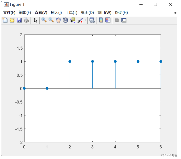
n0=0;nf=6;ns=2;   
n=n0:nf;%生成离散信号的时间序列
f=[zeros(1,ns-n0),ones(1,nf-ns+1)];%生成离散信号f(n)
%也可以用逻辑运算方法产生，f=[(n-ns)>=0]
stem(n,f,'filled'),%填充圆
axis([n0,nf,-2,2])

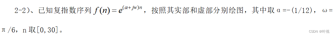
n0=0;nf=30;n=n0:nf;
a=-(1/12);
w=pi/6;
f=exp((a+w*j)*n);
subplot(1,2,1),stem(n,real(f),'filled');
xlabel('n');ylabel('实部');grid
subplot(1,2,2),stem(n,imag(f),'filled');
xlabel('n');ylabel('虚部');grid %填加网格

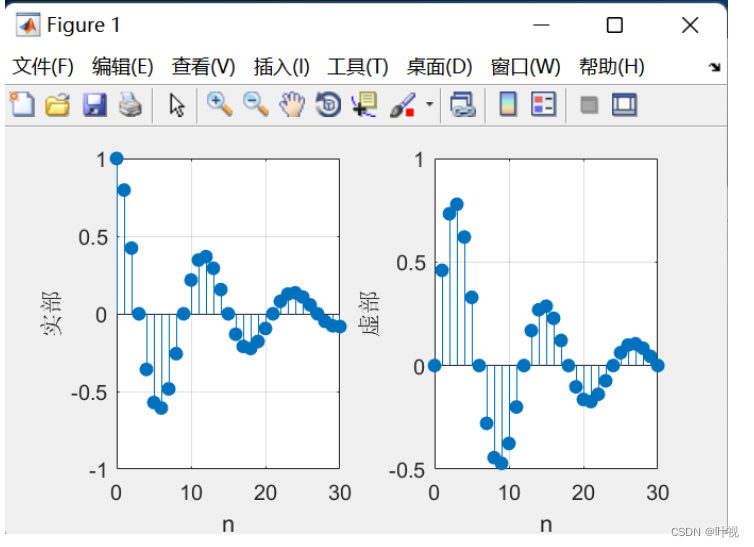
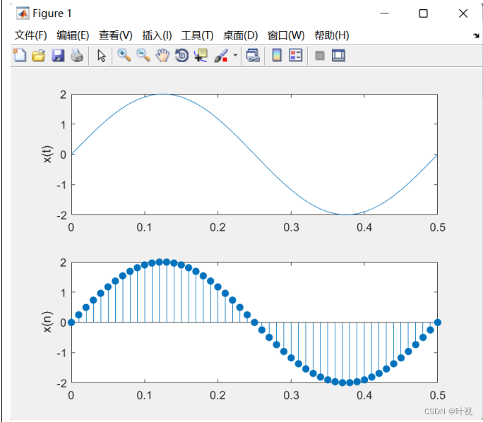
um=2;f=2;nt=1;% 幅值 频率 1个周期
N=50;T=1/f; %50个点  周期
dt=T/N;  % 每个点占的时间
n=0:nt*N;  %建立离散信号的时间序列
tn=n*dt;   %确定时间序列样点在时间轴位置
y=um*sin(2*pi*f.*tn);  %有个点. tn可以看作行项量
subplot(2,1,1);plot(tn,y);
axis([0,nt/2,-2,2]);ylabel('x(t)');
subplot(2,1,2)
stem(tn,y,'filled');%显示经采样的信号
axis([0,nt/2,-2,2]);ylabel('x(n)');

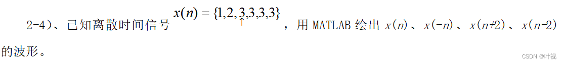
n=[-1:4];
x=[1,2,3,3,3,3];
subplot(2,2,1),stem(n,x,'filled'),grid
subplot(2,2,2),stem((-1)*n,x,'filled'),grid
subplot(2,2,3),stem(n+2,x,'filled'),grid
subplot(2,2,4),stem(n-2,x,'filled'),grid

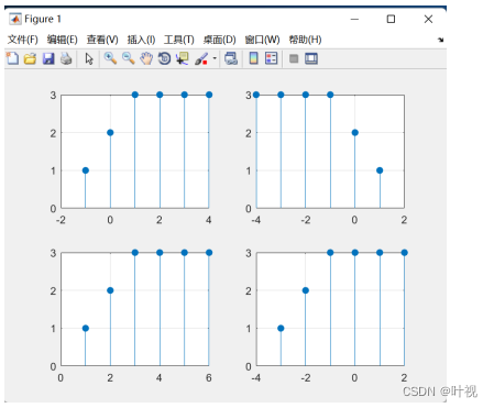
n1=-6:2;f1=[-6 2 0 -5 8 4 3 -1 7];
n2=-2:4; f2=[1 -2 3 0 -3 2 -1];
n=min([n1,n2]):max([n1,n2]);%-6:4   11个
length(n);%11个
x1=zeros(1,length(n));
x2=x1; %x1是都是0的1行10列，x2也都是0的1行10列
x1(find((n>=min(n1))&(n<=max(n1))))=f1;
 %在新序列中放置f1,其中find函数找到索引位置{1，2，3，4，5，6，7，8，9，0，0}
x2(find((n>=min(n2))&(n<=max(n2))))=f2;
 %在新序列中放置f1,其中find函数找到索引位置{0，0，0，0，5，6 ，7，8，9，10，11}
f3=x1+x2;
subplot(2,2,1),stem(n,x1,'filled'),axis([-7,5,-10,10]);title('f1');grid %绘制阶梯图，添加网格
subplot(2,2,2),stem(n,x2,'filled'),axis([-7,5,-4,4]);title('f2');grid
subplot(2,2,3),stem(n,f3,'filled'),axis([-7,5,-10,10]);title('f3');grid

这里是引用

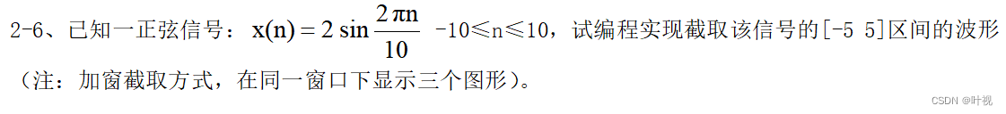
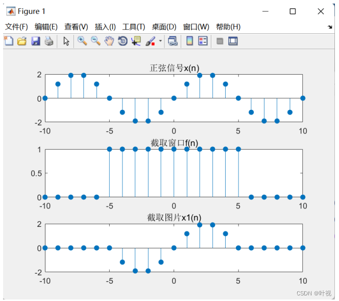
%已知一个正弦信号；-10<=n<=10;试编程截取 [-5 5]的波形
n=-10:10;  
x=2*sin(2*pi*n/10);
f1=[(n+5)>=0]; f2=[(n-5)>0];%逻辑运算
f=f1-f2; %[-5,5]都是1
x1=x.*f; %截取[-5,5]的区间
subplot(311),stem(n,x,'filled'),title('正弦信号x(n)')%绘制阶梯图，添加标题
subplot(312),stem(n,f,'filled'),title('截取窗口f(n)')
subplot(313),stem(n,x1,'filled'),title('截取图片x1(n)')