医疗费用预测模型构建与分析-优快云博客

本文链接：https://blog.youkuaiyun.com/m0_51683462/article/details/125869319

医疗费用预测

笔者的结课作业
[medical cost forecast][https://www.kaggle.com/datasets/mirichoi0218/insurance]

一、数据集探索

在开始之前

df = pd.read_csv('../Data/MedicalCostPersonalDatasets.csv')
df['children'] =df['children'].astype('object')
df

数据集共有1338个样本，包含7个特征，以charge为目标特征。

特征名称	特征说明
age	受益者年龄
sex	保单持有人性别
bmi	身体质量指数（Body Mass Index, BMI)
children	保险计划中所包括的孩子/受抚养着的数量
smoke	被保险人是否吸烟
charge	已经结算的医疗费用

1.居住地与医疗费用的分布

region_cost= df.groupby('region')['charges'].sum() * 1e-6
fig = plt.figure(figsize=(16,8))
sns.barplot(region_cost.index , region_cost.values,color = colors_nude[-1])
plt.title('Region Costs In Million' ,size = 15)
plt.ylabel('In million')
plt.show()

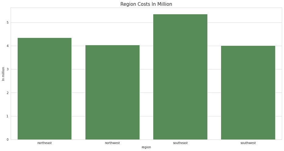
四个地区的charge分布关系southest > northest > nouthwest > southwest

2.年龄与医疗费用的分布

fig = plt.figure(figsize=(16,8))
plt.scatter(df['age'] , df['charges'], cmap = 'summer' ,c = df['bmi'] ,alpha = 0.8 )
plt.xlabel('Age')
plt.ylabel('Charges')
plt.colorbar(label = 'BMI')
plt.title('Age and Charges',size = 15);

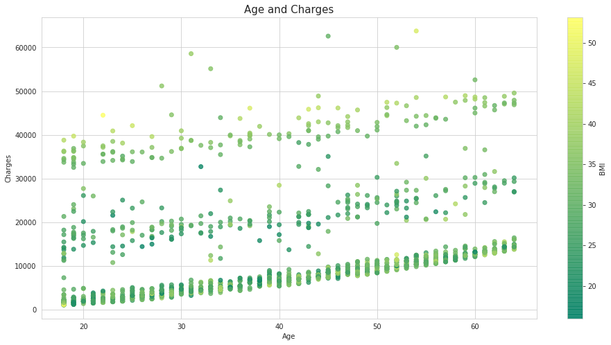
绘制热力图展示相关系数

sns.heatmap(df[['charges' , 'age']].corr(),annot=True, cmap="Greens")

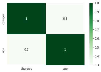
charge与age和BMI均成正相关

3.BMI与Charge的特点分析

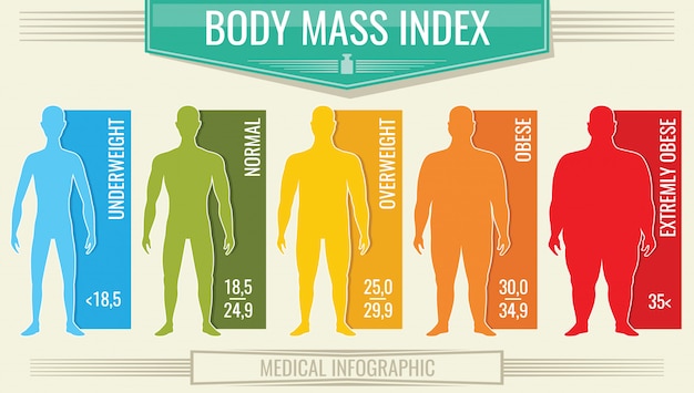
由上图可知在BMI > 35时人便会进入重度肥胖阶段

df.query('bmi > 50 ')['age']

在整个数据集针对BMI，如果采用传统的箱线图其结果并不符合预期，而在本数据集中BMI > 50的仅有3人，我认为这是本数据集中的离群值,故将其删除。

f.drop(df.query('bmi > 50 ').index ,axis= 0 ,inplace=True)
df.drop(df.query('charges > 50000 ').index  ,axis= 0 ,inplace=True)

4.性别与医疗费用的分布

fig = plt.figure(figsize=(16,8))
sns.histplot(data =df[df['sex'] =='male'] ,  x = 'charges' ,color = colors_nude[-1]  ,label = 'male' ,alpha = 0.6)
sns.histplot(data =df[df['sex'] =='female'] ,  x = 'charges',color = colors_nude[1] ,label = 'female' ,alpha = 0.6)
plt.title('Gender Costs',size = 15)
plt.legend()
plt.show()

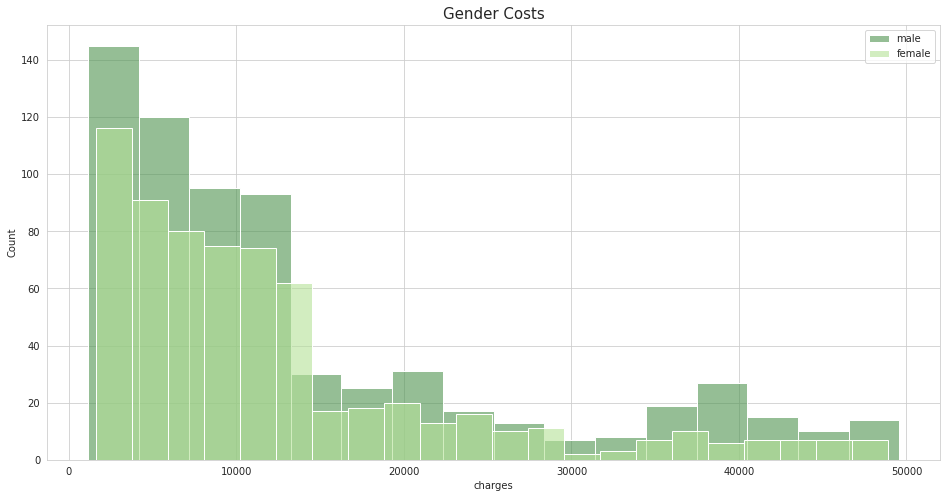
在同等年龄段下男性的医疗花费要大于女性。

5.吸烟与医疗费用的分布

fig  ,ax= plt.subplots(figsize=(16,8))
sns.histplot(data =df[df['smoker'] =='yes'] ,  x = 'charges' ,color = colors_nude[-1]  ,label = 'smoker' ,alpha = 0.6)
sns.histplot(data =df[df['smoker'] =='no'] ,  x = 'charges',color = colors_nude[1] ,label = 'non-smoker' ,alpha = 0.6)
plt.title('smoking Costs',size = 15)
plt.axvline(37000, color="k", linestyle="--");
ax.annotate('here',size = 15, xy(37000,20),xytext(30000,20),arrowprops=dict(arrowstyle="->",connectionstyle="angle3,angleA=0,angleB=-90",color = 'k'));
plt.legend()
plt.show()

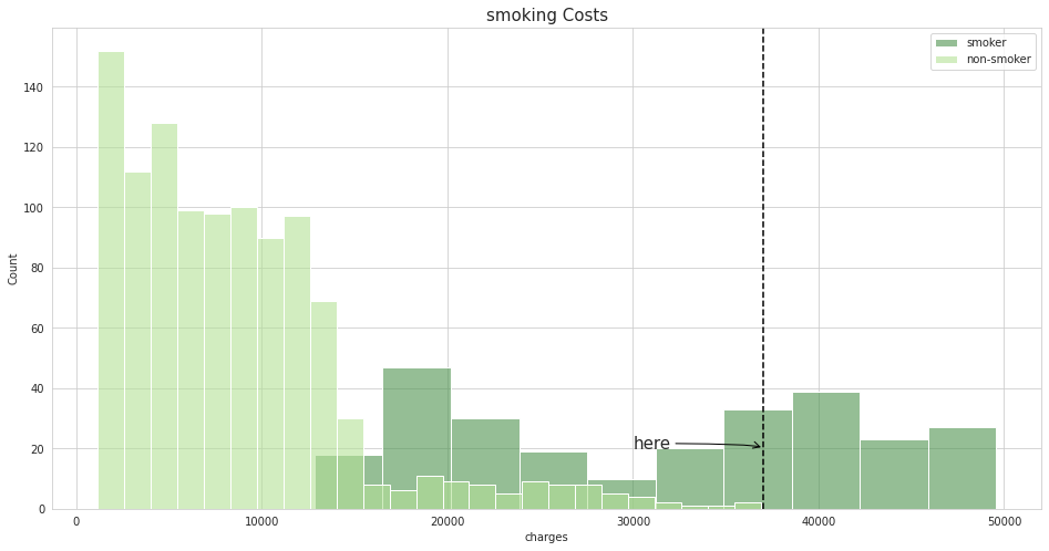
据图，吸烟者的医疗花费要大于不吸烟者,

二、数据清洗

1.缺失值处理

df.nunique()

df.isna().sum()

输出：
	age         0
	sex         0
	bmi         0
	children    0
	smoker      0
	region      0
	charges     0
	dtype: int64

本数据集比较完整无缺失值需要处理。

2.数据去重

df.drop_duplicates(inplace=True)

去除可能存在的重复数据

3.目标变量的分析

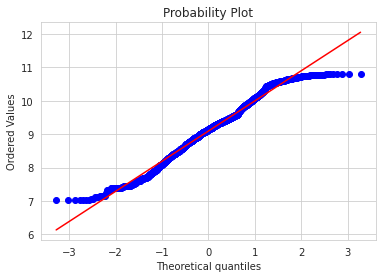
a.分布转换

通过概率分布图和QQ图来展示目标变量charge的分布

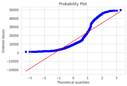
线性回归更加倾向于高斯分布，我们对其取np.log1p() = log（x+1）使其更符合高斯分布

df['charges'] = np.log1p(df['charges'])
sns.distplot(df['charges'] , fit=norm );

(mu, sigma) = norm.fit(df['charges'])
print( '\n mu = {:.2f} and sigma = {:.2f}\n'.format(mu, sigma))

plt.legend(['Normal dist. ($\mu=$ {:.2f} and $\sigma=$ {:.2f} )'.format(mu, sigma)],
            loc='best')
plt.ylabel('Frequency')
plt.title('SalePrice distribution')

fig = plt.figure()
res = stats.probplot(df['charges'], plot=plt )
plt.show()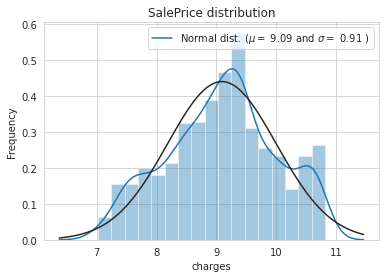

b.多重共线性

线性回归或多元线性回归要求自变量具有很少或没有相似特征

其比较符合预期

三、特征工程

1.训练集与测试机划分

两种切分方式:

随机抽样train_test_split：随机抽取构建训练集与测试集，标签分布不一定一致，适用于较平衡的样本
分层抽样StratifiedShuffleSplit：可以保证训练与测试集中不同标签的分布与原始数据的标签分布基本一致，适用于不平衡样本

这里切分比例为 训练集：测试集 = 8：2

from itertools import combinations
from sklearn.linear_model import LinearRegression
from sklearn.model_selection import train_test_split
cat_col = df.select_dtypes(include = 'object').columns
df = pd.get_dummies(df , cat_col ,drop_first=True)
y =df.pop('charges')
X_train, X_test, y_train, y_test = train_test_split( df , y , test_size=0.2 , random_state=True)

2.多项式创造特征

from sklearn.preprocessing import PolynomialFeatures
poly_features = PolynomialFeatures(degree=3, include_bias=False)
X_train_poly = poly_features.fit_transform(X_train)
X_test_poly=poly_features.transform(X_test)
X_train_poly.shape

效果对比

R-Squared Score without PolynomialFeatures ': 0.7683651933160439

R-Squared Score with PolynomialFeatures': 0.8588104145133237

采用多项式创造特征后的效果明显强于未创造特征

四、模型训练

1.岭回归

RD =Ridge()
RD_param_grid = {'alpha' : [  0.1, 0.12 , 1 ],
                 'solver':['svd']
                }
gsRD = GridSearchCV(RD,param_grid = RD_param_grid, cv=5,scoring="neg_mean_squared_error", n_jobs= 4, verbose = 1)
gsRD.fit(X_train_poly, y_train)
RD_best = gsRD.best_estimator_
RD_best

Fitting 5 folds for each of 3 candidates, totalling 15 fits
Ridge(alpha=1, solver='svd')

2.LASS回归

las =Lasso()
las_param_grid = {'alpha' : [  0.99 ,0.1, 0.12 , 1 ]
                }

gslas = GridSearchCV(las,param_grid = las_param_grid, cv=5,scoring="neg_mean_squared_error", n_jobs= 4, verbose = 1)
gslas.fit(X_train_poly, y_train)
las_best = gslas.best_estimator_
las_best

Fitting 5 folds for each of 4 candidates, totalling 20 fits
Lasso(alpha=0.1)

3.随机森林

RFR =RandomForestRegressor()
RFR_param_grid = {"max_depth": [None],
                    "max_features": [1, 3, 10],
                    "min_samples_split": [2, 3, 10],
                    "min_samples_leaf": [1, 3, 10],
                    "max_leaf_nodes": [ 10 , 16 , 20],
                    "bootstrap": [False],
                    "n_estimators" :[100,300],
                    }
gsRFR = GridSearchCV(RFR,param_grid = RFR_param_grid, cv=5,scoring="neg_mean_squared_error", n_jobs= 4, verbose = 1)
gsRFR.fit(X_train_poly, y_train)
RFR_best = gsRFR.best_estimator_
RFR_best

Fitting 5 folds for each of 162 candidates, totalling 810 fits
RandomForestRegressor(bootstrap=False, max_features=10, max_leaf_nodes=20,
                      min_samples_leaf=3, min_samples_split=10)

4.集成学习梯度提升决策树

GBR = GradientBoostingRegressor()
GBR_param_grid = {
                'n_estimators' : [100,200,300],
                'learning_rate': [0.1, 0.05, 0.01],
                'max_depth': [4, 8],
                'min_samples_leaf': [100,150],
                'max_features': [0.3, 0.1]
}
gsGBR = GridSearchCV(GBR,param_grid = GBR_param_grid, cv=5,scoring="neg_mean_squared_error", n_jobs= 4, verbose = 1)
gsGBR.fit(X_train_poly, y_train)
GBR_best = gsGBR.best_estimator_
GBR_best

Fitting 5 folds for each of 72 candidates, totalling 360 fits
GradientBoostingRegressor(learning_rate=0.05, max_depth=4, max_features=0.1,
                          min_samples_leaf=100, n_estimators=200)

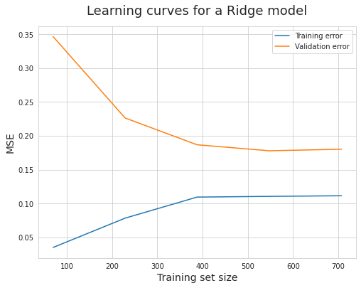
五、绘制学习曲线

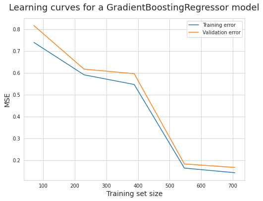
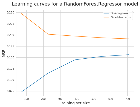
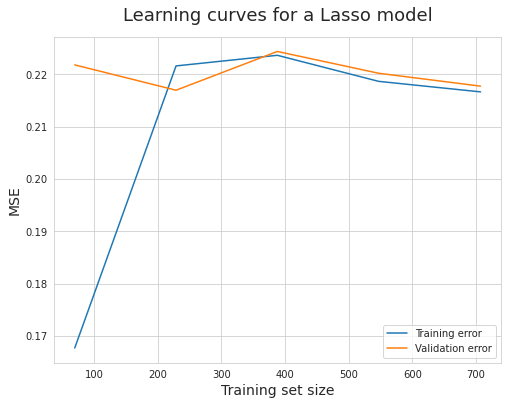
六、最终结果

根据学习曲线可知 $L a sso$ 与 $GradientBoosting $的效果更优, 所以采用$ Lasso$ 与 $GradientBoosting $分别进行本次预测

1. Lasso

Lasso(alpha=0.1)
	Training time: 0.032s
	Prediction time: 0.001s
	Explained variance: 0.7152119815643492
	Mean absolute error: 0.24681562305511537
	R2 score: 0.7152056890004205

2. GradientBoosting

GradientBoostingRegressor(learning_rate=0.05, max_depth=8, max_features=0.3,
                          min_samples_leaf=100)
	Training time: 0.484s
	Prediction time: 0.002s
	Explained variance: 0.8161240496337371
	Mean absolute error: 0.1594930744918336
	R2 score: 0.8159649713544949