【Machine Learning】13.逻辑回归小结and练习

这节回顾一下之前的逻辑回归、正则化的理论知识并实践（光看代码不敲代码可不行啊）

1.导入

import numpy as np
import matplotlib.pyplot as plt
from utils import *
import copy
import math

%matplotlib inline

2.逻辑回归

在这部分练习中，你将建立一个逻辑回归模型来预测学生是否被大学录取。

2.1 问题陈述

假设你是一所大学系的管理员，你想根据两次考试的结果来确定每个申请人的入学机会。

• 您有以前申请者的历史数据，可以用作逻辑回归的培训集。

• 对于每个培训示例，您都有申请人在两次考试中的分数以及录取决定。

• 你的任务是建立一个分类模型，根据这两门考试的分数估计申请者的录取概率。

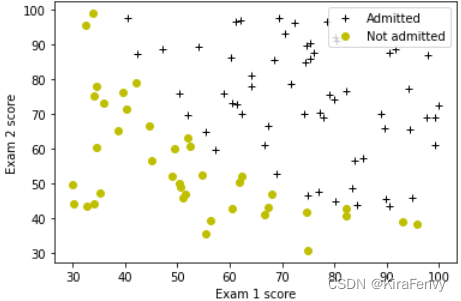
2.2 数据加载和可视化

您将从加载此任务的数据集开始。

• 下面显示的load_dataset（）函数将数据加载到变量X_train和y_train中
• X_train包含学生两次考试的成绩
• “y_train”是录取决定
• y_train=1如果学生被录取
• y_train=0如果学生未被录取
• X_train和`y_train’都是numpy数组。

加载数据

# load dataset
X_train, y_train = load_data("data/ex2data1.txt")

熟悉一下数据集

print("First five elements in X_train are:\n", X_train[:5]) #查看前五条数据
print("Type of X_train:",type(X_train))


First five elements in X_train are:
 [[34.62365962 78.02469282]
 [30.28671077 43.89499752]
 [35.84740877 72.90219803]
 [60.18259939 86.3085521 ]
 [79.03273605 75.34437644]]
Type of X_train: <class 'numpy.ndarray'>

print("First five elements in y_train are:\n", y_train[:5])
print("Type of y_train:",type(y_train))

First five elements in y_train are:
 [0. 0. 0. 1. 1.]
Type of y_train: <class 'numpy.ndarray'>

print ('The shape of X_train is: ' + str(X_train.shape))
print ('The shape of y_train is: ' + str(y_train.shape))
print ('We have m = %d training examples' % (len(y_train)))

The shape of X_train is: (100, 2)
The shape of y_train is: (100,)
We have m = 100 training examples

数据可视化

# Plot examples
plot_data(X_train, y_train[:], pos_label="Admitted", neg_label="Not admitted")

# Set the y-axis label
plt.ylabel('Exam 2 score') 
# Set the x-axis label
plt.xlabel('Exam 1 score') 
plt.legend(loc="upper right")
plt.show()

2.3 Sigmoid函数

$$f_{\mathbf{w},b}(x)=g(\mathbf{w}\cdot \mathbf{x}+b)$$

$$g(z)=\frac{1}{1+e^{-z}}$$

Exercise 1

Please complete the sigmoid function to calculate

$$g(z)=\frac{1}{1+e^{-z}}$$

Note that

• z 不一定是一个数，也可以是一个数组
• 如果输入时数组，要对每个sigmoid函数应用值
• 记得np.exp()的使用

def sigmoid(z):
    """
    Compute the sigmoid of z

    Args:
        z (ndarray): A scalar, numpy array of any size.

    Returns:
        g (ndarray): sigmoid(z), with the same shape as z
         
    """
    g = 1/(1+(np.exp(-z)))
    
    return g

2.4 逻辑回归的代价函数 Cost function for logistic regression

Exercise 2

Please complete the compute_cost function using the equations below.

Recall that for logistic regression, the cost function is of the form

$$J(\mathbf{w},b)=\frac{1}{m}\sum _{i=0}^{m-1}\left[loss(f_{\mathbf{w},b}({\mathbf{x}}^{(i)}),y^{(i)})\right]\text{\hspace{1em}(1)}$$

where

• m is the number of training examples in the dataset

• $loss(f_{\mathbf{w},b}({\mathbf{x}}^{(i)}),y^{(i)})$ is the cost for a single data point, which is -

  $$loss(f_{\mathbf{w},b}({\mathbf{x}}^{(i)}),y^{(i)})=(-y^{(i)}\log \left(f_{\mathbf{w},b}\left({\mathbf{x}}^{(i)}\right)\right)-\left(1-y^{(i)}\right)\log \left(1-f_{\mathbf{w},b}\left({\mathbf{x}}^{(i)}\right)\right)\text{\hspace{1em}(2)}$$

• $f_{\mathbf{w},b}({\mathbf{x}}^{(i)})$ is the model’s prediction, while $y^{(i)}$, which is the actual label

• $f_{\mathbf{w},b}({\mathbf{x}}^{(i)})=g(\mathbf{w}\cdot {\mathbf{x}}^{(\mathbf{i})}+b)$ where function $g$ is the sigmoid function.

  • It might be helpful to first calculate an intermediate variable $z_{\mathbf{w},b}({\mathbf{x}}^{(i)})=\mathbf{w}\cdot {\mathbf{x}}^{(\mathbf{i})}+b=w_0{x}_0^{(i)}+...+w_{n-1}{x}_{n-1}^{(i)}+b$ where $n$ is the number of features, before calculating $f_{\mathbf{w},b}({\mathbf{x}}^{(i)})=g(z_{\mathbf{w},b}({\mathbf{x}}^{(i)}))$

Note:

• As you are doing this, remember that the variables X_train and y_train are not scalar values but matrices of shape ($m,n$) and ($m$,1) respectively, where $n$ is the number of features and $m$ is the number of training examples.
• You can use the sigmoid function that you implemented above for this part.
• numpy有np.log()

def compute_cost(X, y, w, b, lambda_= 1):
    """
    Computes the cost over all examples
    Args:
      X : (ndarray Shape (m,n)) data, m examples by n features
      y : (array_like Shape (m,)) target value 
      w : (array_like Shape (n,)) Values of parameters of the model      
      b : scalar Values of bias parameter of the model
      lambda_: unused placeholder
    Returns:
      total_cost: (scalar)         cost 
    """

    m, n = X.shape
    loss_sum = 0
    ### START CODE HERE ###
    for i in range(m):
      z_wb = 0
      for j in range(n):
        z_wb_xi = w[j] * X[i][j]
        z_wb += z_wb_xi

      z_wb += b
      f_wb = sigmoid(z_wb)
      loss = -y[i] * np.log(f_wb) - (1-y[i]) * np.log(1-f_wb)
      loss_sum += loss

    total_cost = loss_sum/m
    ### END CODE HERE ### 
    
    return total_cost

代码测试

m, n = X_train.shape

# Compute and display cost with w initialized to zeroes
initial_w = np.zeros(n)
initial_b = 0.
cost = compute_cost(X_train, y_train, initial_w, initial_b)
print('Cost at initial w (zeros): {:.3f}'.format(cost))

Cost at initial w (zeros): 0.693

2.5 逻辑回归的梯度计算

梯度下降函数
repeat until convergence:    {    b : = b − α ∂ J ( w , b ) ∂ b    w j : = w j − α ∂ J ( w , b ) ∂ w j    for j := 0..n-1 } \begin{align*}& \text{repeat until convergence:} \; \lbrace \newline \; & b := b - \alpha \frac{\partial J(\mathbf{w},b)}{\partial b} \newline \; & w_j := w_j - \alpha \frac{\partial J(\mathbf{w},b)}{\partial w_j} \tag{1} \; & \text{for j := 0..n-1}\newline & \rbrace\end{align*} ​repeat until convergence:{b:=b−α∂b∂J(w,b)​wj​:=wj​−α∂wj​∂J(w,b)​}​for j := 0..n-1​(1)​

Exercise 3

Please complete the compute_gradient function to compute $\frac{\partial J(\mathbf{w},b)}{\partial w}$, $\frac{\partial J(\mathbf{w},b)}{\partial b}$ from equations (2) and (3) below.

$$\frac{\partial J(\mathbf{w},b)}{\partial b}=\frac{1}{m}\sum _{i=0}^{m-1}(f_{\mathbf{w},b}({\mathbf{x}}^{(i)})-{\mathbf{y}}^{(i)})\text{\hspace{1em}(2)}$$
$$\frac{\partial J(\mathbf{w},b)}{\partial w_j}=\frac{1}{m}\sum _{i=0}^{m-1}(f_{\mathbf{w},b}({\mathbf{x}}^{(i)})-{\mathbf{y}}^{(i)})x_j^{(i)}\text{\hspace{1em}(3)}$$

• m is the number of training examples in the dataset
• $f_{\mathbf{w},b}(x^{(i)})$ is the model’s prediction, while $y^{(i)}$ is the actual label

• Note: While this gradient looks identical to the linear regression gradient, the formula is actually different because linear and logistic regression have different definitions of $f_{\mathbf{w},b}(x)$.

# UNQ_C3
# GRADED FUNCTION: compute_gradient
def compute_gradient(X, y, w, b, lambda_=None): 
    """
    Computes the gradient for logistic regression 
 
    Args:
      X : (ndarray Shape (m,n)) variable such as house size 
      y : (array_like Shape (m,1)) actual value 
      w : (array_like Shape (n,1)) values of parameters of the model      
      b : (scalar)                 value of parameter of the model 
      lambda_: unused placeholder.
    Returns
      dj_dw: (array_like Shape (n,1)) The gradient of the cost w.r.t. the parameters w. 
      dj_db: (scalar)                The gradient of the cost w.r.t. the parameter b. 
    """
    m, n = X.shape
    dj_dw = np.zeros(w.shape)
    dj_db = 0.

    ### START CODE HERE ### 
    diff = 0.  # 浮点数
    for i in range(m):
      z_wb = 0.
      for j in range(n):
        z_wb+=w[j] * X[i][j]
      # 不要忘了加回b
      z_wb += b
      f_wb = sigmoid(z_wb)
      # 上述计算可简化为f_wb_i = sigmoid(np.dot(X[i],w) + b)
      dj_db_i = f_wb - y[i]
      dj_dw_ij = 0.
      for j in range(n):
        dj_dw[j] = dj_dw[j]+dj_db_i*X[i][j] # 关键的实现语句
      dj_db += dj_db_i


    dj_db /=m
    dj_dw /= m

    ### END CODE HERE ###

        
    return dj_db, dj_dw

代码测试

# Compute and display gradient with w initialized to zeroes
initial_w = np.zeros(n)
initial_b = 0.

dj_db, dj_dw = compute_gradient(X_train, y_train, initial_w, initial_b)
print(f'dj_db at initial w (zeros):{dj_db}' )
print(f'dj_dw at initial w (zeros):{dj_dw.tolist()}' )

dj_db at initial w (zeros):-0.1
dj_dw at initial w (zeros):[-12.00921658929115, -11.262842205513591]

2.6 通过梯度下降学习参数

验证梯度下降是否正常工作的一个好方法是查看$J（\mathbf{w}，b）$，检查它是否随每个步骤而减少，直到某个值不动

def gradient_descent(X, y, w_in, b_in, cost_function, gradient_function, alpha, num_iters, lambda_): 
    """
    Performs batch gradient descent to learn theta. Updates theta by taking 
    num_iters gradient steps with learning rate alpha
    
    Args:
      X :    (array_like Shape (m, n)
      y :    (array_like Shape (m,))
      w_in : (array_like Shape (n,))  Initial values of parameters of the model
      b_in : (scalar)                 Initial value of parameter of the model
      cost_function:                  function to compute cost
      alpha : (float)                 Learning rate
      num_iters : (int)               number of iterations to run gradient descent
      lambda_ (scalar, float)         regularization constant
      
    Returns:
      w : (array_like Shape (n,)) Updated values of parameters of the model after
          running gradient descent
      b : (scalar)                Updated value of parameter of the model after
          running gradient descent
    """
    
    # number of training examples
    m = len(X)
    
    # An array to store cost J and w's at each iteration primarily for graphing later
    J_history = []
    w_history = []
    
    for i in range(num_iters):

        # Calculate the gradient and update the parameters
        dj_db, dj_dw = gradient_function(X, y, w_in, b_in, lambda_)   

        # Update Parameters using w, b, alpha and gradient
        w_in = w_in - alpha * dj_dw               
        b_in = b_in - alpha * dj_db              
       
        # Save cost J at each iteration
        if i<100000:      # prevent resource exhaustion 
            cost =  cost_function(X, y, w_in, b_in, lambda_)
            J_history.append(cost)

        # Print cost every at intervals 10 times or as many iterations if < 10
        if i% math.ceil(num_iters/10) == 0 or i == (num_iters-1):
            w_history.append(w_in)
            print(f"Iteration {i:4}: Cost {float(J_history[-1]):8.2f}   ")
        
    return w_in, b_in, J_history, w_history #return w and J,w history for graphing

代码测试

np.random.seed(1)
intial_w = 0.01 * (np.random.rand(2).reshape(-1,1) - 0.5)
initial_b = -8


# Some gradient descent settings
iterations = 10000
alpha = 0.001

w,b, J_history,_ = gradient_descent(X_train ,y_train, initial_w, initial_b, 
                                   compute_cost, compute_gradient, alpha, iterations, 0)


Iteration    0: Cost     1.01   
Iteration 1000: Cost     0.31   
Iteration 2000: Cost     0.30   
Iteration 3000: Cost     0.30   
Iteration 4000: Cost     0.30   
Iteration 5000: Cost     0.30   
Iteration 6000: Cost     0.30   
Iteration 7000: Cost     0.30   
Iteration 8000: Cost     0.30   
Iteration 9000: Cost     0.30  

2.7 绘制决策边界

def plot_decision_boundary(w, b, X, y):
    # Credit to dibgerge on Github for this plotting code
     
    plot_data(X[:, 0:2], y)
    
    if X.shape[1] <= 2:
        plot_x = np.array([min(X[:, 0]), max(X[:, 0])])
        plot_y = (-1. / w[1]) * (w[0] * plot_x + b)
        
        plt.plot(plot_x, plot_y, c="b")
        
    else:
        u = np.linspace(-1, 1.5, 50)
        v = np.linspace(-1, 1.5, 50)
        
        z = np.zeros((len(u), len(v)))

        # Evaluate z = theta*x over the grid
        for i in range(len(u)):
            for j in range(len(v)):
                z[i,j] = sig(np.dot(map_feature(u[i], v[j]), w) + b)
        
        # important to transpose z before calling contour       
        z = z.T
        
        # Plot z = 0
        plt.contour(u,v,z, levels = [0.5], colors="g")


plot_decision_boundary(w, b, X_train, y_train)

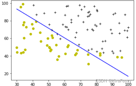
2.8 模型评估

我们可以通过观察所学模型对训练集的预测程度来评估我们发现的参数的质量。

Exercise 4

Please complete the predict function to produce 1 or 0 predictions given a dataset and a learned parameter vector $w$ and $b$.

• First you need to compute the prediction from the model $f(x^{(i)})=g(w\cdot x^{(i)})$ for every example

  • You’ve implemented this before in the parts above

• We interpret the output of the model ($f(x^{(i)})$) as the probability that $y^{(i)}=1$ given $x^{(i)}$ and parameterized by $w$.

• Therefore, to get a final prediction ($y^{(i)}=0$ or $y^{(i)}=1$) from the logistic regression model, you can use the following heuristic -

  if $f(x^{(i)})>=0.5$, predict $y^{(i)}=1$

  if $f(x^{(i)})<0.5$, predict $y^{(i)}=0$

def predict(X, w, b): 
    """
    Predict whether the label is 0 or 1 using learned logistic
    regression parameters w
    
    Args:
    X : (ndarray Shape (m, n))
    w : (array_like Shape (n,))      Parameters of the model
    b : (scalar, float)              Parameter of the model

    Returns:
    p: (ndarray (m,1))
        The predictions for X using a threshold at 0.5
    """
    # number of training examples
    m, n = X.shape   
    p = np.zeros(m)
   
    ### START CODE HERE ### 
    for i in range(m):
        f_xi = sigmoid(np.dot(X[i],w)+b)
        if f_xi >= 0.5:
            p[i] = 1
        else:
            p[i] = 0
        
    ### END CODE HERE ### 
    return p

代码测试

# Test your predict code
np.random.seed(1)
tmp_w = np.random.randn(2)
tmp_b = 0.3    
tmp_X = np.random.randn(4, 2) - 0.5

tmp_p = predict(tmp_X, tmp_w, tmp_b)
print(f'Output of predict: shape {tmp_p.shape}, value {tmp_p}')


Output of predict: shape (4,), value [0. 1. 1. 1.]
All tests passed!

计算训练集的accuracy

#Compute accuracy on our training set
p = predict(X_train, w,b)
print('Train Accuracy: %f'%(np.mean(p == y_train) * 100))


Train Accuracy: 92.000000

3. 正则化的逻辑回归

在这部分练习中，您将实施正规化逻辑回归，以预测来自制造厂的微芯片是否通过质量保证（QA）。在QA过程中，每个微芯片都要经过各种测试，以确保其正常工作。

3.1 Problem Statement

假设你是工厂的产品经理，你有一些芯片在两个不同测试中的测试结果。

• 从这两个测试中，您想确定微芯片应该被接受还是拒绝。
• 为了帮助你做出决定，你有一个关于过去芯片测试结果的数据集，从中你可以建立一个逻辑回归模型。

3.2 加载和可视化数据

与本练习前面的部分类似，让我们从加载此任务的数据集并将其可视化开始。

• 下面显示的load_dataset（）函数将数据加载到变量X_train和y_train中
• “X_train”包含两次测试的微芯片测试结果
• “y_train”包含QA结果
• y_train=1如果微芯片被接受
• y_train=0如果芯片被拒绝
• X_train和`y_train’都是numpy数组。

加载训练数据

def load_data(filename):
    data = np.loadtxt(filename, delimiter=',')
    X = data[:,:2]
    y = data[:,2]
    return X, y
    
# load dataset
X_train, y_train = load_data("data/ex2data2.txt")

检查数据（一般会检查前五条数据，数据类型和维度）

# print X_train
print("X_train:", X_train[:5])
print("Type of X_train:",type(X_train))

# print y_train
print("y_train:", y_train[:5])
print("Type of y_train:",type(y_train))

X_train: [[ 0.051267  0.69956 ]
 [-0.092742  0.68494 ]
 [-0.21371   0.69225 ]
 [-0.375     0.50219 ]
 [-0.51325   0.46564 ]]
Type of X_train: <class 'numpy.ndarray'>
y_train: [1. 1. 1. 1. 1.]
Type of y_train: <class 'numpy.ndarray'>

print ('The shape of X_train is: ' + str(X_train.shape))
print ('The shape of y_train is: ' + str(y_train.shape))
print ('We have m = %d training examples' % (len(y_train)))

The shape of X_train is: (118, 2)
The shape of y_train is: (118,)
We have m = 118 training examples

数据可视化

def plot_data(X, y, pos_label="y=1", neg_label="y=0"):
    positive = y == 1
    negative = y == 0
    
    # Plot examples
    plt.plot(X[positive, 0], X[positive, 1], 'k+', label=pos_label)
    plt.plot(X[negative, 0], X[negative, 1], 'yo', label=neg_label)

# Plot examples
plot_data(X_train, y_train[:], pos_label="Accepted", neg_label="Rejected")

# Set the y-axis label
plt.ylabel('Microchip Test 2') 
# Set the x-axis label
plt.xlabel('Microchip Test 1') 
plt.legend(loc="upper right")
plt.show()

3.3 特征映射

更好地拟合数据的一种方法是从每个数据点创建更多特征。在提供的函数“map_feature”中，我们将把特征映射到$x_1$和$x_2$的所有多项式项，直到六次方。

$$map\_feature(x)=\left[\begin{array}{c}{x}_1\\ x_2\\ x_1^2\\ x_1{x}_2\\ x_2^2\\ x_1^3\\ ⋮\\ x_1{x}_2^5\\ x_2^6\end{array}\right]$$

由于这种映射，我们的两个特征向量（两次QA测试的分数）已转换为27维向量。在这个高维特征向量上训练的逻辑回归分类器将具有更复杂的决策边界，并且在我们的二维图中绘制时将是非线性的。

def map_feature(X1, X2):
    """
    Feature mapping function to polynomial features    
    """
    X1 = np.atleast_1d(X1)
    X2 = np.atleast_1d(X2)
    degree = 6
    out = []
    for i in range(1, degree+1):
        for j in range(i + 1):
            out.append((X1**(i-j) * (X2**j)))
    return np.stack(out, axis=1)

函数调用

print("Original shape of data:", X_train.shape)

mapped_X =  map_feature(X_train[:, 0], X_train[:, 1])
print("Shape after feature mapping:", mapped_X.shape)

Original shape of data: (118, 2)
Shape after feature mapping: (118, 27)

查看变化前后的第一个元素

print("X_train[0]:", X_train[0])
print("mapped X_train[0]:", mapped_X[0])

X_train[0]: [0.051267 0.69956 ]
mapped X_train[0]: [5.12670000e-02 6.99560000e-01 2.62830529e-03 3.58643425e-02
 4.89384194e-01 1.34745327e-04 1.83865725e-03 2.50892595e-02
 3.42353606e-01 6.90798869e-06 9.42624411e-05 1.28625106e-03
 1.75514423e-02 2.39496889e-01 3.54151856e-07 4.83255257e-06
 6.59422333e-05 8.99809795e-04 1.22782870e-02 1.67542444e-01
 1.81563032e-08 2.47750473e-07 3.38066048e-06 4.61305487e-05
 6.29470940e-04 8.58939846e-03 1.17205992e-01]

虽然特征映射允许我们构建更具表现力的分类器，但它也更容易出现过拟合。在练习的下一部分中，您将实现正则化逻辑回归以拟合数据，并亲自了解正则化如何帮助解决过拟合问题。

3.4 正则化逻辑回归的代价函数

Recall that for regularized logistic regression, the cost function is of the form
$$J(\mathbf{w},b)=\frac{1}{m}\sum _{i=0}^{m-1}\left[-y^{(i)}\log \left(f_{\mathbf{w},b}\left({\mathbf{x}}^{(i)}\right)\right)-\left(1-y^{(i)}\right)\log \left(1-f_{\mathbf{w},b}\left({\mathbf{x}}^{(i)}\right)\right)\right]+\frac{\lambda }{2m}\sum _{j=0}^{n-1}{w}_j^2$$

Compare this to the cost function without regularization (which you implemented above), which is of the form

$$J(\mathbf{w}.b)=\frac{1}{m}\sum _{i=0}^{m-1}\left[(-y^{(i)}\log \left(f_{\mathbf{w},b}\left({\mathbf{x}}^{(i)}\right)\right)-\left(1-y^{(i)}\right)\log \left(1-f_{\mathbf{w},b}\left({\mathbf{x}}^{(i)}\right)\right)\right]$$

The difference is the regularization term, which is $$\frac{\lambda }{2m}\sum _{j=0}^{n-1}{w}_j^2$$
Note that the $b$ parameter is not regularized.

Exercise 5

Please complete the compute_cost_reg function below to calculate the following term for each element in $w$
$$\frac{\lambda }{2m}\sum _{j=0}^{n-1}{w}_j^2$$

The starter code then adds this to the cost without regularization (which you computed above in compute_cost) to calculate the cost with regulatization.

def compute_cost_reg(X, y, w, b, lambda_ = 1):
    """
    Computes the cost over all examples
    Args:
      X : (array_like Shape (m,n)) data, m examples by n features
      y : (array_like Shape (m,)) target value 
      w : (array_like Shape (n,)) Values of parameters of the model      
      b : (array_like Shape (n,)) Values of bias parameter of the model
      lambda_ : (scalar, float)    Controls amount of regularization
    Returns:
      total_cost: (scalar)         cost 
    """

    m, n = X.shape
    
    # Calls the compute_cost function that you implemented above
    cost_without_reg = compute_cost(X, y, w, b) 
    
    # You need to calculate this value
    reg_cost = 0.
    
    ### START CODE HERE ###
    for j in range(n):
      reg_cost += w[j]*w[j]
        
    ### END CODE HERE ### 
    
    # Add the regularization cost to get the total cost
    total_cost = cost_without_reg + (lambda_/(2 * m)) * reg_cost

    return total_cost

测试

X_mapped = map_feature(X_train[:, 0], X_train[:, 1])
np.random.seed(1)
initial_w = np.random.rand(X_mapped.shape[1]) - 0.5
initial_b = 0.5
lambda_ = 0.5
cost = compute_cost_reg(X_mapped, y_train, initial_w, initial_b, lambda_)

print("Regularized cost :", cost)


Regularized cost : 0.6618252552483948

3.5 正则化后的梯度计算

The gradient of the regularized cost function has two components. The first, $\frac{\partial J(\mathbf{w},b)}{\partial b}$ is a scalar, the other is a vector with the same shape as the parameters $\mathbf{w}$, where the $j^{\mathrm{th}}$ element is defined as follows:

$$\frac{\partial J(\mathbf{w},b)}{\partial b}=\frac{1}{m}\sum _{i=0}^{m-1}(f_{\mathbf{w},b}({\mathbf{x}}^{(i)})-y^{(i)})$$

$$\frac{\partial J(\mathbf{w},b)}{\partial w_j}=\left(\frac{1}{m}\sum _{i=0}^{m-1}(f_{\mathbf{w},b}({\mathbf{x}}^{(i)})-y^{(i)})x_j^{(i)}\right)+\frac{\lambda }{m}{w}_j$$

Compare this to the gradient of the cost function without regularization (which you implemented above), which is of the form
$$\frac{\partial J(\mathbf{w},b)}{\partial b}=\frac{1}{m}\sum _{i=0}^{m-1}(f_{\mathbf{w},b}({\mathbf{x}}^{(i)})-{\mathbf{y}}^{(i)})\text{\hspace{1em}(2)}$$
$$\frac{\partial J(\mathbf{w},b)}{\partial w_j}=\frac{1}{m}\sum _{i=0}^{m-1}(f_{\mathbf{w},b}({\mathbf{x}}^{(i)})-{\mathbf{y}}^{(i)})x_j^{(i)}\text{\hspace{1em}(3)}$$

As you can see,$\frac{\partial J(\mathbf{w},b)}{\partial b}$ is the same, the difference is the following term in $\frac{\partial J(\mathbf{w},b)}{\partial w}$, which is $$\frac{\lambda }{m}{w}_j$$

Please complete the compute_gradient_reg function below to modify the code below to calculate the following term

$$\frac{\lambda }{m}{w}_j$$

The starter code will add this term to the $\frac{\partial J(\mathbf{w},b)}{\partial w}$ returned from compute_gradient above to get the gradient for the regularized cost function.

def compute_gradient_reg(X, y, w, b, lambda_ = 1): 
    """
    Computes the gradient for linear regression 
 
    Args:
      X : (ndarray Shape (m,n))   variable such as house size 
      y : (ndarray Shape (m,))    actual value 
      w : (ndarray Shape (n,))    values of parameters of the model      
      b : (scalar)                value of parameter of the model  
      lambda_ : (scalar,float)    regularization constant
    Returns
      dj_db: (scalar)             The gradient of the cost w.r.t. the parameter b. 
      dj_dw: (ndarray Shape (n,)) The gradient of the cost w.r.t. the parameters w. 

    """
    m, n = X.shape
    
    dj_db, dj_dw = compute_gradient(X, y, w, b)

    ### START CODE HERE ###     
    dj_dw += lambda_*w/m
        
    ### END CODE HERE ###         
        
    return dj_db, dj_dw

代码测试

X_mapped = map_feature(X_train[:, 0], X_train[:, 1])
np.random.seed(1) 
initial_w  = np.random.rand(X_mapped.shape[1]) - 0.5 
initial_b = 0.5
 
lambda_ = 0.5
dj_db, dj_dw = compute_gradient_reg(X_mapped, y_train, initial_w, initial_b, lambda_)

print(f"dj_db: {dj_db}", )
print(f"First few elements of regularized dj_dw:\n {dj_dw[:4].tolist()}", )

dj_db: 0.07138288792343662
First few elements of regularized dj_dw:
 [-0.010386028450548701, 0.011409852883280124, 0.0536273463274574, 0.003140278267313462]

3.6 通过梯度下降学习参数

变化在梯度计算和代价计算当中，这里直接调用梯度下降函数

# Initialize fitting parameters
np.random.seed(1)
initial_w = np.random.rand(X_mapped.shape[1])-0.5
initial_b = 1.

# Set regularization parameter lambda_ to 1 (you can try varying this)
lambda_ = 0.01;                                          
# Some gradient descent settings
iterations = 10000
alpha = 0.01

w,b, J_history,_ = gradient_descent(X_mapped, y_train, initial_w, initial_b, 
                                    compute_cost_reg, compute_gradient_reg, 
                                    alpha, iterations, lambda_)

Iteration    0: Cost     0.72   
Iteration 1000: Cost     0.59   
Iteration 2000: Cost     0.56   
Iteration 3000: Cost     0.53   
Iteration 4000: Cost     0.51   
Iteration 5000: Cost     0.50   
Iteration 6000: Cost     0.48   
Iteration 7000: Cost     0.47   
Iteration 8000: Cost     0.46   
Iteration 9000: Cost     0.45   
Iteration 9999: Cost     0.45  

3.7 绘制决策边界

plot_decision_boundary(w, b, X_mapped, y_train)

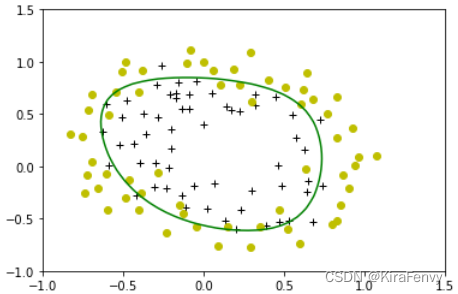
3.8 评估正则化后的模型

准确率

#Compute accuracy on the training set
p = predict(X_mapped, w, b)

print('Train Accuracy: %f'%(np.mean(p == y_train) * 100))


Train Accuracy: 82.203390