数据分析实例2 (英文报告)-确定性价比最高的汽油种类（不同行驶条件）-R语言 Linear Regression-Kaggle 数据

Find Economical Gas by Using Multiple Linear Regression

AIWEN XING, YU ZHANG
 

1 Abstract

Authors used multiple linear regression on the gas consumption data and to find factors that affect the consumption of two kinds of gas, E10, and SP98, significantly. By doing data transformation on the predictor variables and response, authors got a more reasonable model and did the model diagnostic. The final predictor for E10 should be speed and temperature, and that for SP98 should be speed, temperature and it is rainy or not. The result is that E10 is economical at low speed while SP98 is economical in high speed and rain affects consumption of both types.

2 Introduction

It is common that adding Ethanol into gasoline for environmental protection. Super Plus, 95 with 10%, added Ethanol was called as SP95/E10 in Eurozone, which is abbreviated as E10 in following contents. These two kinds of gas, E10, and Super Plus 98 (SP98) are all available in gas stations. E10 is cheaper than SP98 in one unit. However, it is said that E10 reduces fuel economy of vehicles. So, E10 may cause more fuel costs than SP98 does under some conditions.
 
Based on this statement, this project tried to discover which factors affect the gas consumption and how they influence the consumption. The project also tried to discuss which gas is more economical.

The authors are interested in one data set, car fuel consumption, that was published at Kaggle.com. The data set documented gas consumption of two types gas (E10, and SP98) on one car that driving by one driver under different conditions.

3 Analysis Process

3.1 Preliminary Analysis

The original dataset contains 258 observations, one response, and six variables. The variables and its meaning are listed in Table 1.

Table 1 Variables and description in gas consumption dataset

The authors split raw data into two subsets named E10 and SP98. Analyzing gas consumption by gas types is convenient. E10 has 120 observations. SP98 has 138 observations.

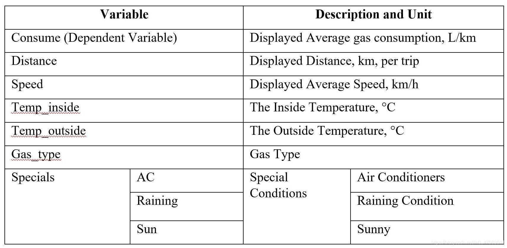
The scatter matrix, Figure 1 and Figure 2, of response (consume), reveals that some variables may have correlations and data transformation might be applied for getting better distribution plots.

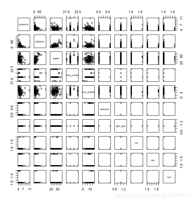
Figure 1 Scatterplot matrix for gas E10 consumption

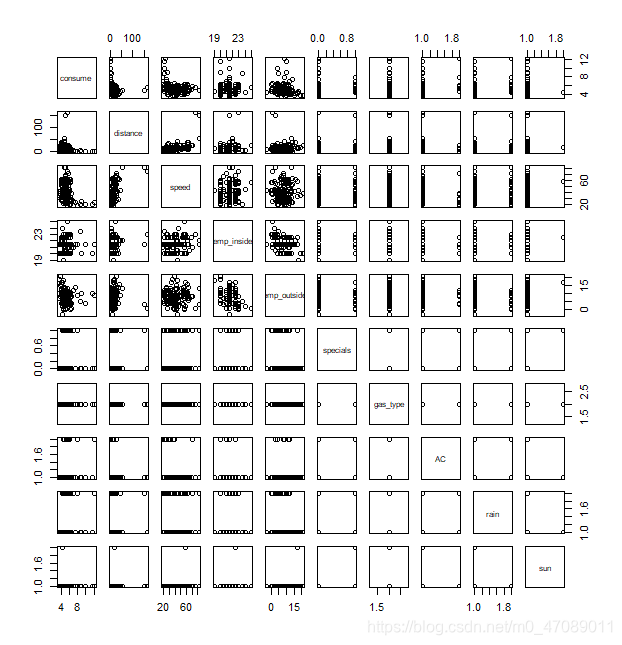
Figure 2 Scatterplot matrix for gas SP98 consumption
 
3.1.1 Replacement of Missing Values
There are nine missing values of inside temperature in raw data SP98. The missing data are replaced as the median value (21.5) of interior temperature.

3.1.2 Analysis of Correlations of Predictors
Table 2 shows the correlation coefficient of predictors. The correlation between speed and distance is 0.53, so the predictor SPEED is highly correlated to predictor DISTANCE. Speed represents the displayed average speed of each one-way route, and the average speed was measured by the distance in a given period. Although some values of distance in the data set are the same, the average speed is not exactly same. For example, when driving in downtown or near residential communities, there are more stop signs and traffic lights, so it causes the increasing spent time. Hence, the values of average speed are various in the same distance.

The correlation between inside temperature (Temp_inside) and outside temperature (Temp_outside) is -0.18. However, it does not mean that Temp_inside are correlated to Temp_outside. However, the correlation does not imply causation. The outside temperature of a vehicle does not affect the final inside temperature. There are only four levels of Temp_inside: 21, 21.5, 22, and 22.5. The standard deviation of Temp_inside (0.471605) is small. It causes the calculated correlation gets a large value that does not indicate correlations between Temp_inside and Temp_outside. So, they can be considered as independent variables. The rest values of correlation are too small to be considered.
Table 2 Correlation efficient of variables in dataset

	Distance	Speed	Temp_indise	Temp_outside
Distance	1	0.53	0.10	-0.005
Speed	0.53	1	0.11	0.03
Temp_inside	0.10	0.11	1	-0.18
Temp_outside	-0.005	0.03	-0.18	1

The authors applied the multiple linear regression to find an appropriate model. Details of the regression are described in later paragraphs.

3.1.3 Data Transformation
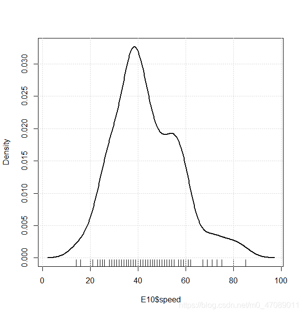
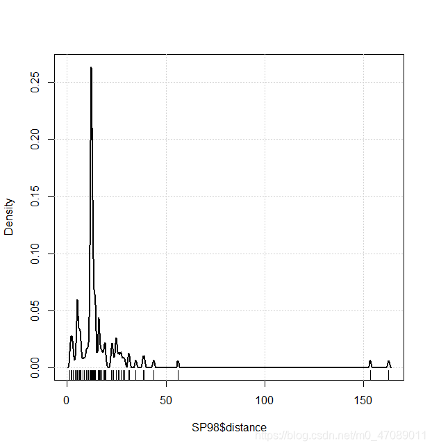
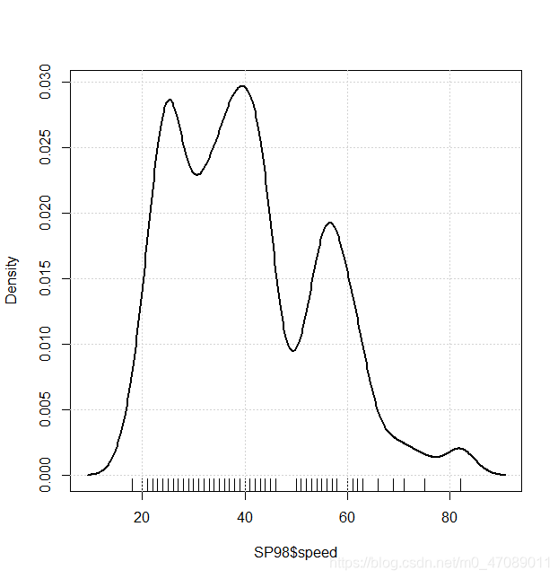
Distance and Speed are continuous variables. Their Distributions are neither symmetric nor normality in Figure 3.The authors centralized data and transferred data by logarithm. The distributions after transformation are shown in Figure 5.

(3a)

(3b)

(3c)

(3d)
Figure 3 Density plot of distance and speed in E10 and SP98

3.1.3 (a) Data Centralization
To comply data centralization, the raw data abstract an appropriate constant that closes to modes of variables. The abstraction values and modes values are documented in Table 3.
Table 3 Mode and abstraction value in E10 and SP98

Data Set $ Variable	Mode	Abstraction Value
E10$Distance	12.3	12.0