


opencv系列-图像配准
前言:配准方面的知识,在工作中多有用到,对于原理了解一些,但是知之不深,最近时间比较充裕,专门写一篇文章,加深对配准方面知识的学习。
一、简介
通俗定义:给定两幅图像P1,P2,图像配准算法的目标是找到一种变换T: Ω 1 \Omega1 Ω1 Ω 2 \Omega2 Ω2,使得变换某一图后,两幅图像的相似程度达到最大。
二、应用场景
Panorama全景拼接;recognition识别;SLAM(同步定位与地图绘制);去噪;hdr算法
三、算法分类
Feature based; Optical Flow based;CNN based
四、特征点
特征检测。手动或者可能自动检测显著和独特的对象(闭合边界区域,边缘,轮廓,交线,角点等)。为了进一步处理,这些特征可以通过点来表示(重心,线尾,特征点),这些点称为控制点(CP)。
特征匹配。建立场景图像和参考图像特征之间的相关性。使用各种各样的特征描述符,相似性度量,连同特征的空间相关性。
转换模型估计。估计将感测图像和参考图像对齐的所谓映射函数的类型和参数。映射函数的参数通过特征相关性计算。
图像重采样和转换。使用映射函数转换感测图像。使用合适的插值技术计算非整数坐标的图像值。
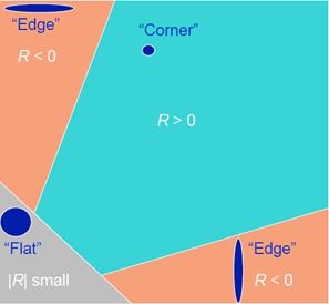
4.1 Haris
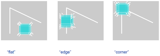
window fuction: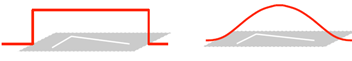
SIFT
SURF
五、特征匹配
Opencv特征寻找及匹配的步骤有哪些?
- 根据特征点定义寻找特征点
- 对特征点进行描述
- 将寻找到的关键点和现有特征点,利用描述符进行量化后,进行匹配。
六、全局配准
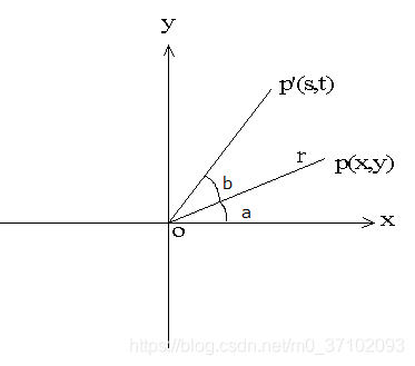
坐标旋转变换公式的推导
围绕原点的旋转
s
=
r
∗
c
o
s
(
b
+
a
)
=
r
∗
c
o
s
(
a
)
∗
c
o
s
(
b
)
−
r
∗
s
i
n
(
a
)
∗
s
i
n
(
b
)
s = r*cos(b+a) = r*cos(a)*cos(b) - r*sin(a)*sin(b)
s=r∗cos(b+a)=r∗cos(a)∗cos(b)−r∗sin(a)∗sin(b)
t
=
r
∗
s
i
n
(
b
+
a
)
=
r
∗
s
i
n
(
b
)
∗
c
o
s
(
a
)
+
r
∗
s
i
n
(
a
)
∗
c
o
s
(
b
)
t = r*sin(b+a) = r*sin(b)*cos(a) +r*sin(a)*cos(b)
t=r∗sin(b+a)=r∗sin(b)∗cos(a)+r∗sin(a)∗cos(b)
x
=
r
∗
c
o
s
(
a
)
x = r*cos(a)
x=r∗cos(a)
y
=
r
∗
s
i
n
(
a
)
y = r*sin(a)
y=r∗sin(a)
将x,y带入s,y当中:
s
=
x
∗
c
o
s
(
b
)
−
y
∗
s
i
n
(
b
)
s = x*cos(b) - y*sin(b)
s=x∗cos(b)−y∗sin(b)
t
=
x
∗
s
i
n
(
b
)
+
y
∗
c
o
s
(
b
)
t = x*sin(b) + y*cos(b)
t=x∗sin(b)+y∗cos(b)
写成矩阵的形式:
[
s
t
]
=
[
c
o
s
(
b
)
−
s
i
n
(
b
)
s
i
n
(
b
)
c
o
s
(
b
)
]
[
x
y
]
\begin{bmatrix} s \\ t \end{bmatrix} =\begin{bmatrix} cos(b) & -sin(b) \\ sin(b) & cos(b) \end{bmatrix} \begin{bmatrix} x \\ y \end{bmatrix}
[st]=[cos(b)sin(b)−sin(b)cos(b)][xy]
坐标系(逆时针)的旋转
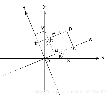
以P点坐标为例,在原始坐标系中坐标是(x,y),在新的坐标系中的坐标为(s,t)
s
=
o
s
=
o
a
+
a
s
=
y
∗
s
i
n
(
θ
)
+
x
∗
c
o
s
(
θ
)
s = os = oa + as = y*sin(\theta) + x*cos(\theta)
s=os=oa+as=y∗sin(θ)+x∗cos(θ)
t
=
o
t
=
a
y
−
b
y
=
y
∗
c
o
s
(
θ
)
−
x
∗
s
i
n
(
θ
)
t = ot = ay - by = y*cos(\theta) - x*sin(\theta)
t=ot=ay−by=y∗cos(θ)−x∗sin(θ)
写成矩阵的形式:
[
s
t
]
=
[
c
o
s
(
θ
)
s
i
n
(
θ
)
−
s
i
n
(
θ
)
c
o
s
(
θ
)
]
[
x
y
]
\begin{bmatrix} s \\ t \end{bmatrix} = \begin{bmatrix} cos(\theta) & sin(\theta) \\ -sin(\theta) & cos(\theta) \end{bmatrix} \begin{bmatrix} x \\ y \end{bmatrix}
[st]=[cos(θ)−sin(θ)sin(θ)cos(θ)][xy]
绕某一点进行旋转
待补充
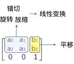
仿射变换
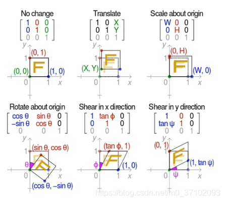
仿射变换(Affine Transformation or Affine Map),在几何上,是一个向量空间,经过线性变换和平移转换为另外一个向量空间的操作。仿射变换的特点,保持图像的平移性(直线仍然是直的)和平行性(平行线仍然平行,且直线点上的位置顺序不变)。
常见的三种变换操作:
- 旋转(rotation)
坐标系顺时针,内容逆时针
[ c o s ( θ ) − s i n ( θ ) s i n ( θ ) c o s ( θ ) ] [ x y ] = [ x 1 y 1 ] \begin{bmatrix} cos(\theta) & - sin(\theta) \\ sin(\theta) & cos(\theta) \end{bmatrix} \begin{bmatrix} x \\ y \end{bmatrix} = \begin{bmatrix} x_{1} \\ y_{1} \end{bmatrix} [cos(θ)sin(θ)−sin(θ)cos(θ)][xy]=[x1y1] - 平移(translation)
[ 1 0 T x 0 1 T y 0 0 1 ] [ X Y 1 ] = [ X + T x Y + T y 1 ] \begin{bmatrix} 1 & 0 & T_{x} \\ 0 & 1 & T_{y} \\ 0 & 0 & 1 \end{bmatrix} \begin{bmatrix} X \\ Y \\ 1 \end{bmatrix} = \begin{bmatrix} X + T_{x} \\ Y + T_{y} \\ 1 \end{bmatrix} ⎣⎡100010TxTy1⎦⎤⎣⎡XY1⎦⎤=⎣⎡X+TxY+Ty1⎦⎤ - 缩放(scale)
[ T x 0 0 0 T y 0 0 0 1 ] [ X Y 1 ] = [ X ∗ T x Y ∗ T y 1 ] \begin{bmatrix}T_{x} & 0 & 0 & \\ 0 & T_{y} & 0 \\ 0 & 0 & 1 \end{bmatrix} \begin{bmatrix} X \\ Y \\ 1 \end{bmatrix} = \begin{bmatrix} X * T_{x} \\ Y *T_{y} \\ 1 \end{bmatrix} ⎣⎡Tx000Ty0001⎦⎤⎣⎡XY1⎦⎤=⎣⎡X∗TxY∗Ty1⎦⎤ - 错切(shear)
x轴移动
[ 1 t a n θ 0 0 1 0 0 0 1 ] [ X Y 1 ] = [ X + Y ∗ t a n θ Y 1 ] \begin{bmatrix}1 & tan\theta & 0 & \\ 0 & 1 & 0 \\ 0 & 0 & 1 \end{bmatrix} \begin{bmatrix} X \\ Y \\ 1 \end{bmatrix} = \begin{bmatrix} X +Y*tan\theta \\ Y \\ 1 \end{bmatrix} ⎣⎡100tanθ10001⎦⎤⎣⎡XY1⎦⎤=⎣⎡X+Y∗tanθY1⎦⎤
y轴移动
[ 1 0 0 t a n α 1 0 0 0 1 ] [ X Y 1 ] = [ X Y + X ∗ t a n α 1 ] \begin{bmatrix}1 & 0 & 0 & \\ tan\alpha & 1 & 0 \\ 0 & 0 & 1 \end{bmatrix} \begin{bmatrix} X \\ Y \\ 1 \end{bmatrix} = \begin{bmatrix} X \\ Y + X*tan\alpha \\ 1 \end{bmatrix} ⎣⎡1tanα0010001⎦⎤⎣⎡XY1⎦⎤=⎣⎡XY+X∗tanα1⎦⎤
x、y轴移动
[ 1 t a n θ 0 t a n α 1 0 0 0 1 ] [ X Y 1 ] = [ X + Y ∗ t a n θ Y + X ∗ t a n α 1 ] \begin{bmatrix}1 & tan\theta & 0 & \\ tan\alpha & 1 & 0 \\ 0 & 0 & 1 \end{bmatrix} \begin{bmatrix} X \\ Y \\ 1 \end{bmatrix} = \begin{bmatrix} X +Y*tan\theta \\ Y + X*tan\alpha \\ 1 \end{bmatrix} ⎣⎡1tanα0tanθ10001⎦⎤⎣⎡XY1⎦⎤=⎣⎡X+Y∗tanθY+X∗tanα1⎦⎤
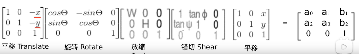
A
=
[
a
00
a
01
a
10
a
11
]
B
=
[
b
00
b
10
]
M
=
[
A
B
]
A = \begin{bmatrix} a_{00} & a_{01} \\ a_{10} & a_{11} \\ \end{bmatrix} B=\begin{bmatrix} b_{00} \\ b_{10} \\ \end{bmatrix} M=\begin{bmatrix} A& B \end{bmatrix}
A=[a00a10a01a11]B=[b00b10]M=[AB]
T
=
A
∗
[
x
y
]
+
B
或
者
T
=
M
∗
[
x
y
1
]
T = A*\begin{bmatrix} x \\ y \\ \end{bmatrix} +B 或者 T = M*\begin{bmatrix} x \\ y \\ 1\end{bmatrix}
T=A∗[xy]+B或者T=M∗⎣⎡xy1⎦⎤
对于图片的每个位置进行转换:
T
=
[
a
00
∗
x
+
a
01
∗
y
+
b
00
a
10
∗
x
+
a
11
∗
y
+
b
10
]
T = \begin{bmatrix} a_{00}*x + a_{01}*y +b_{00} \\ a_{10}*x + a_{11}*y +b_{10} \end{bmatrix}
T=[a00∗x+a01∗y+b00a10∗x+a11∗y+b10]
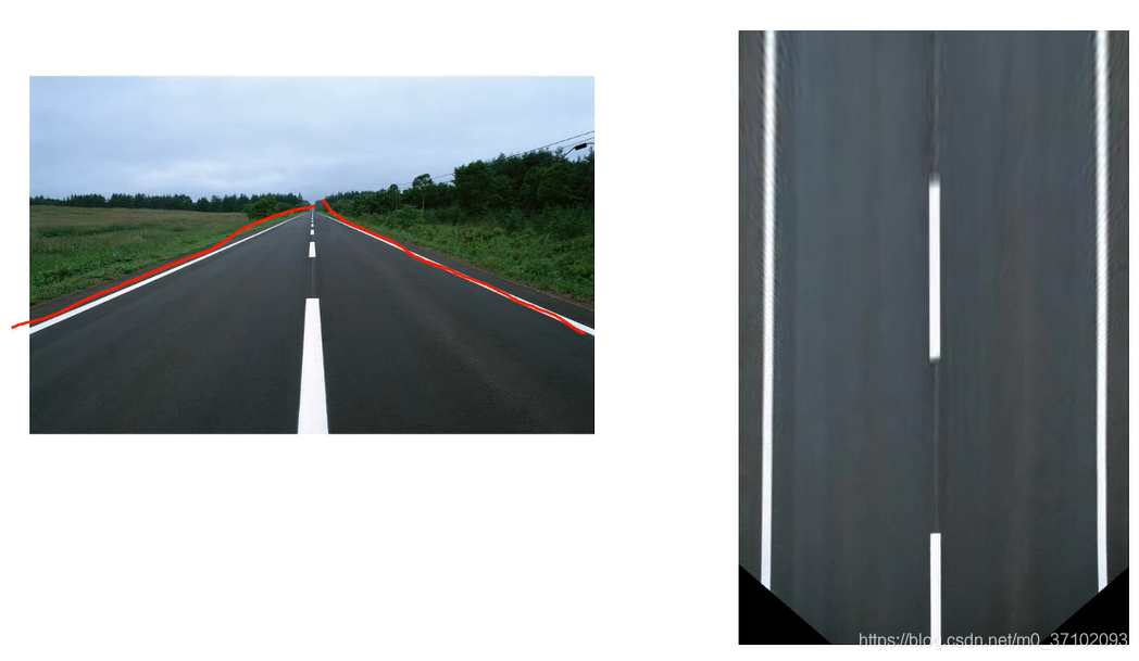
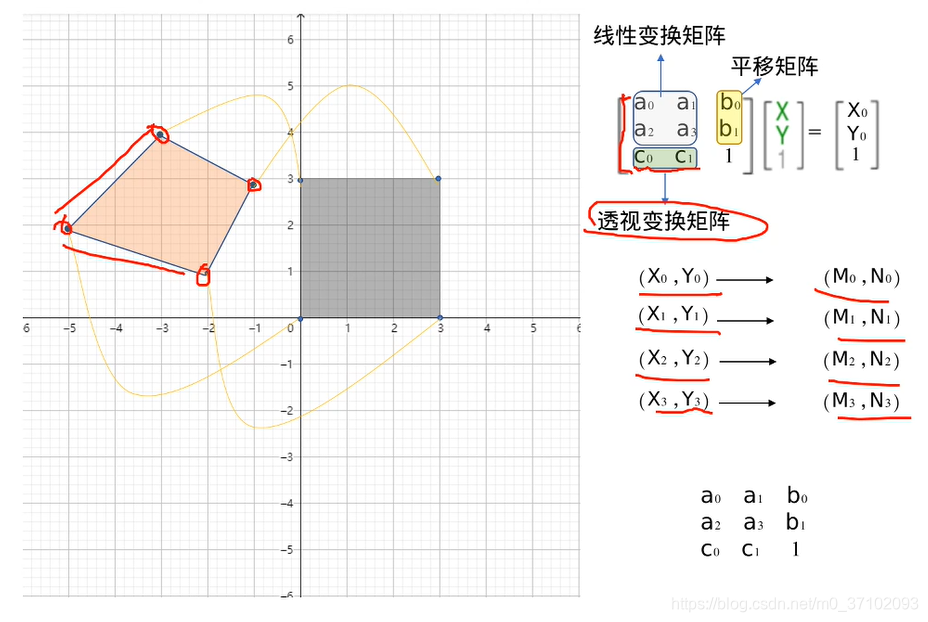
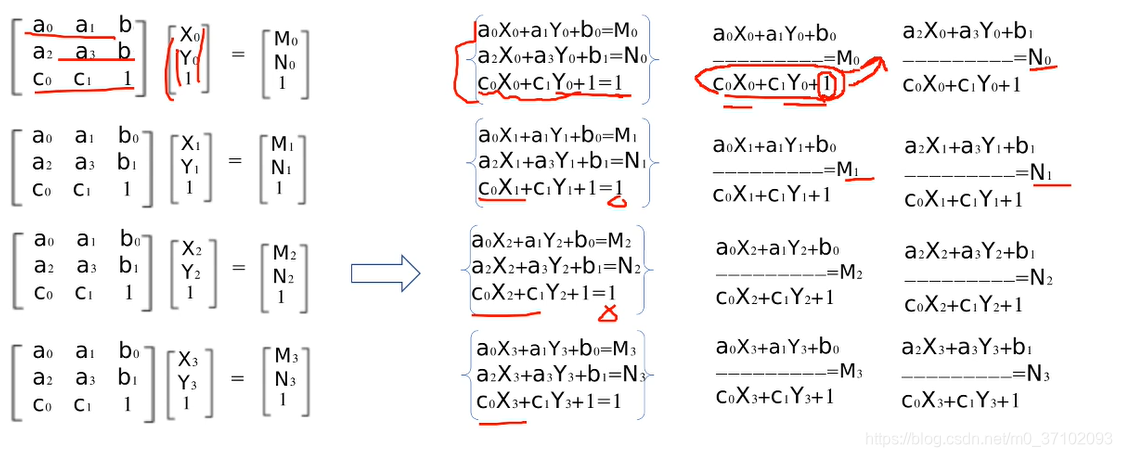
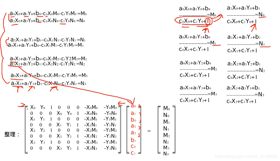
透视变换与仿射变换
opencv函数使用
什么是光流(optical flow)?
所谓光流即瞬时速度,时间很小时,等同于目标点的位移。
光流的物理意义:光流是由目标物体的运动以及相机的运动,或者二者共同的运动所产生。研究光流场的目的是为了获得运动场。
光流法基本原理
七、 局部配准
-[8]surf特征提取算法


 60
60

 被折叠的 条评论
为什么被折叠?
被折叠的 条评论
为什么被折叠?
 到【灌水乐园】发言


