吴恩达机器学习作业一python实现

最新推荐文章于 2024-04-10 20:43:42 发布

lyp_1020k

最新推荐文章于 2024-04-10 20:43:42 发布

阅读量781

点赞数 1

分类专栏：机器学习线性回归文章标签： python

本文链接：https://blog.youkuaiyun.com/lyp_1020k/article/details/109539095

版权

机器学习同时被 2 个专栏收录

2 篇文章

订阅专栏

线性回归

1 篇文章

订阅专栏

这篇博客介绍了吴恩达机器学习课程中的单变量线性回归，通过Python实现数据处理，包括读入数据并查看统计量，以及绘制数据散点图。博主使用梯度下降法优化代价函数，求得最佳参数θ，并进行了结果的可视化展示。

摘要生成于 C知道，由 DeepSeek-R1 满血版支持，前往体验 >

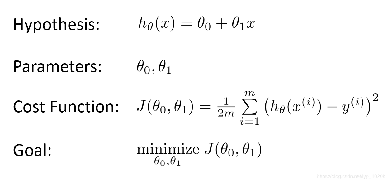
单变量线性回归

参考了黄海广的github：https://github.com/fengdu78/Coursera-ML-AndrewNg-Notes

数据处理

读入数据

path = 'ex1data1.txt'
data = pd.read_csv(path, names=['Population', 'Profit'])

可查看数据的一些统计量

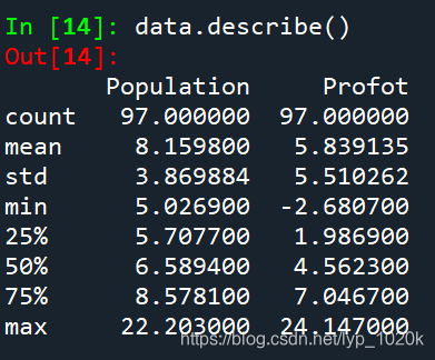
图：数据的一些统计量

展示数据

data.plot(kind='scatter', x='Population', y='Profit', figsize=(12,8))
plt.show()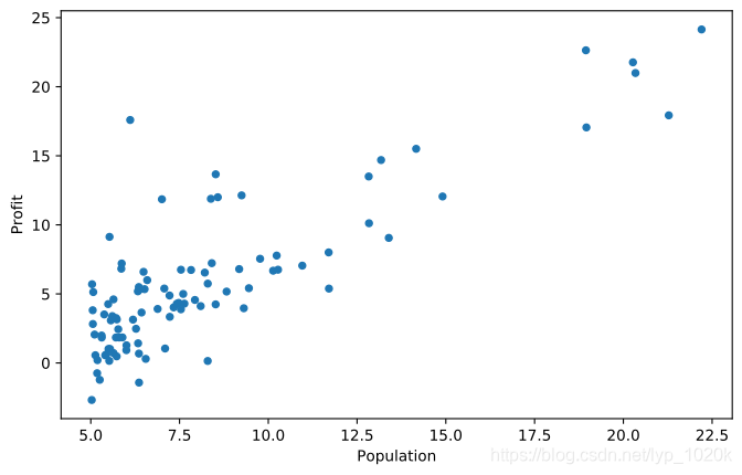

图：原数据的散点图

梯度下降

代价函数

公式：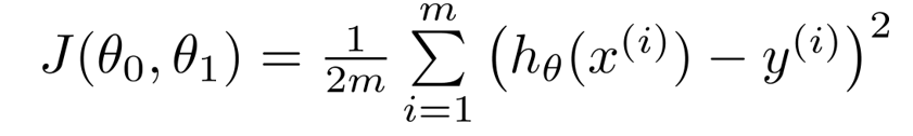

# 计算代价函数J(θ)
def cost_function(X, y, theta):
    diff = X.dot(theta.T) - y
    return sum(np.power(diff, 2))/(2*m)

梯度下降法

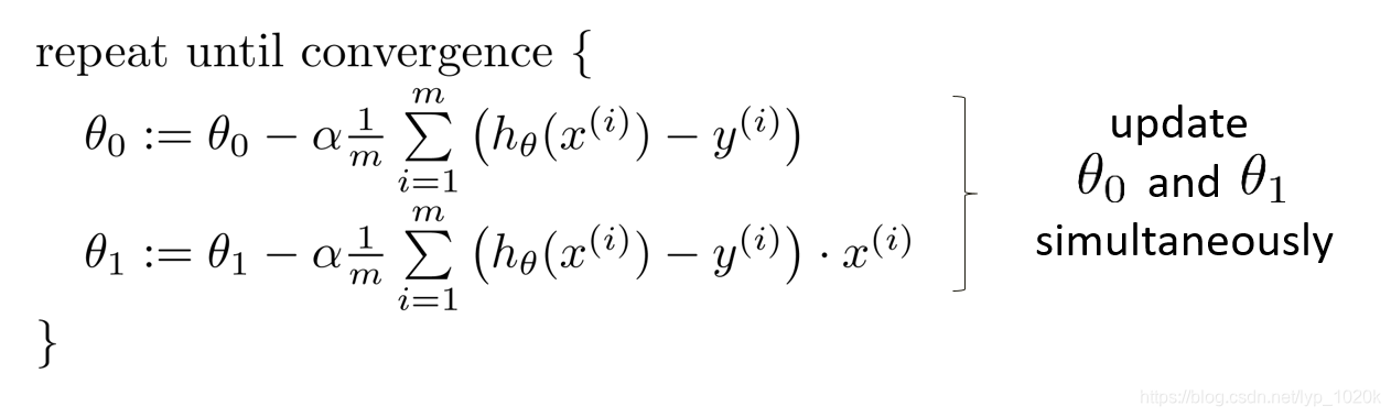
对θ0和θ1求偏导

# 求偏导
def gradient_function(X, y, theta):
    diff = X.dot(theta.T) - y
    return diff.dot(X)/m

梯度下降

def gradient_descent(X, y, alpha):
    theta = np.array((m,1)) 
    gradient = gradient_function(X, y, theta)
    while not all (abs(gradient) <= 1e-5):
        theta = theta - alpha * gradient
        gradient = gradient_function(X, y, theta)
    return theta

找到的最佳的θ

进行可视化

population = np.linspace(data.Population.min(), data.Population.max(), 100) # 横坐标
profit = optimal_theta[0] + (optimal_theta[1] * population) # 纵坐标

fig, ax = plt.subplots(figsize=(8, 6))
ax.plot(population, profit, 'r', label='Prediction')
ax.scatter(data['Population'], data['Profit'], label='Training data')
ax.legend(loc=4) # 4表示标签在右下角
ax.set_xlabel('Population')
ax.set_ylabel('Profit')
ax.set_title('Prediction Profit by. Population Size')
plt.show()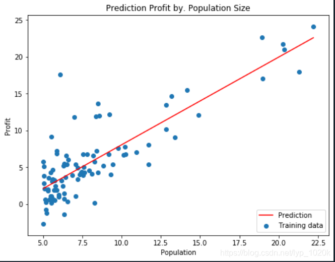

源码：

import numpy as np
import pandas as pd
import matplotlib.pyplot as plt

path = 'ex1data1.txt'
data = pd.read_csv(path, names=['Population', 'Profit'])

m = len(data)
data.plot(kind='scatter', x='Population', y='Profit', figsize=(12,8))



# 计算代价函数J(θ)
def cost_function(X, y, theta):
    diff = X.dot(theta.T) - y
    return sum(np.power(diff, 2))/(2*m)

# 求偏导
def gradient_function(X, y, theta):
    diff = X.dot(theta.T) - y
    return diff.dot(X)/m

# 梯度下降
def gradient_descent(X, y, alpha):
    theta = np.array((m,1)) 
    gradient = gradient_function(X, y, theta)
    while not all (abs(gradient) <= 1e-5):
        theta = theta - alpha * gradient
        gradient = gradient_function(X, y, theta)
    return theta

X = data['Population']
y = data['Profit']
X = np.vstack((pd.Series(np.ones(m)), X)).T
alpha = 0.01

optimal_theta = gradient_descent(X, y, alpha)
print('optimal_theta:', optimal_theta)

population = np.linspace(data.Population.min(), data.Population.max(), 100) # 横坐标
profit = optimal_theta[0] + (optimal_theta[1] * population) # 纵坐标

fig, ax = plt.subplots(figsize=(8, 6))
ax.plot(population, profit, 'r', label='Prediction')
ax.scatter(data['Population'], data['Profit'], label='Training data')
ax.legend(loc=4) # 4表示标签在右下角
ax.set_xlabel('Population')
ax.set_ylabel('Profit')
ax.set_title('Prediction Profit by. Population Size')
plt.show()

本人刚开始学，才疏学浅