Faster RCNN-1（RPN）

Faster RCNN是个很经典的two-stage目标检测网络，也是一年多以前我接触到的第一个深度学习网络。现在结合着github上大神复现的pytorch源码认真研读一下。博客仅做自己的理解和笔记。
参考文章：https://zhuanlan.zhihu.com/p/31426458 ，这篇是我看过的最好的介绍Faster RCNN的文章。
github代码地址：https://github.com/jwyang/faster-rcnn.pytorch ，框架用的是pytorch

RPN的结构

可以看到RPN网络实际分为2条线，上面一条通过softmax分类anchors获得foreground和background（检测目标是foreground），下面一条用于计算对于anchors的bounding box regression偏移量，以获得精确的proposal。而最后的Proposal层则负责综合foreground anchors和bounding box regression偏移量获取proposals，同时剔除太小和超出边界的proposals。其实整个网络到了Proposal Layer这里，就完成了相当于目标定位的功能。
也可以参考caffe网络结构生成的图

在代码中lib/rpn文件夹的目录结构是这样的

• rpn.py 定义了RPN网络的整个流程。
• proposal_layer.py 在 rpn.py 文件中被调用，生成了一系列符合要求的anchor（见后面内容）

# for each (H, W) location i
        #   generate A anchor boxes centered on cell i
        #   apply predicted bbox deltas at cell i to each of the A anchors
        # clip predicted boxes to image
        # remove predicted boxes with either height or width < threshold
        # sort all (proposal, score) pairs by score from highest to lowest
        # take top pre_nms_topN proposals before NMS
        # apply NMS with threshold 0.7 to remaining proposals
        # take after_nms_topN proposals after NMS
        # return the top proposals (-> RoIs top, scores top)

• generate_anchors.py 在 proposal _layer.py 中被调用，用来对每个像素点生成4*9的向量（9个anchor，每个anchor输出x,y,w,h四个坐标）
• anchor_target_layer 对每个anchor生成类别标签和bbox Regression targets，返回 rpn.py 中中计算loss

RPN流程

一副MxN大小的矩阵送入Faster RCNN网络后，到RPN网络变为(M/16)x(N/16)，不妨设 W=M/16，H=N/16。
首先经过3x3卷积，通道数为512，变为512xWxH
然后分为两条路，经过两个1x1卷积，通道数分别变为18和36
卷积核定义如下：

    # define the convrelu layers processing input feature map
    self.RPN_Conv = nn.Conv2d(self.din, 512, 3, 1, 1, bias=True)   # input size = output size

    # define bg/fg classifcation score layer
    self.nc_score_out = len(self.anchor_scales) * len(self.anchor_ratios) * 2 # 2(bg/fg) * 9 (anchors)
    self.RPN_cls_score = nn.Conv2d(512, self.nc_score_out, 1, 1, 0)

    # define anchor box offset prediction layer
    self.nc_bbox_out = len(self.anchor_scales) * len(self.anchor_ratios) * 4 # 4(coords) * 9 (anchors)
    self.RPN_bbox_pred = nn.Conv2d(512, self.nc_bbox_out, 1, 1, 0)

    # define proposal layer
    self.RPN_proposal = _ProposalLayer(self.feat_stride, self.anchor_scales, self.anchor_ratios)

    # define anchor target layer
    self.RPN_anchor_target = _AnchorTargetLayer(self.feat_stride, self.anchor_scales, self.anchor_ratios)

rpn.py的forward（）函数如下：

     batch_size = base_feat.size(0)

    # return feature map after convrelu layer
    rpn_conv1 = F.relu(self.RPN_Conv(base_feat), inplace=True)              # (1, 512, H, W)
    # get rpn classification score
    rpn_cls_score = self.RPN_cls_score(rpn_conv1)                           # (1, 2*9, H, W)

    rpn_cls_score_reshape = self.reshape(rpn_cls_score, 2)                  # (1, 2*9, H, W)->(1, 2, 9*H, W)
    rpn_cls_prob_reshape = F.softmax(rpn_cls_score_reshape, 1)
    rpn_cls_prob = self.reshape(rpn_cls_prob_reshape, self.nc_score_out)    # (1, 2, 9*H, W)->(1, 2*9, H, W)

    # get rpn offsets to the anchor boxes
    rpn_bbox_pred = self.RPN_bbox_pred(rpn_conv1)                           # (1, 512, H, W)->(1, 4*9, H, W)

    # proposal layer
    cfg_key = 'TRAIN' if self.training else 'TEST'

    rois = self.RPN_proposal((rpn_cls_prob.data, rpn_bbox_pred.data,
                             im_info, cfg_key))

    self.rpn_loss_cls = 0
    self.rpn_loss_box = 0

    # generating training labels and build the rpn loss
    if self.training:
        assert gt_boxes is not None

        rpn_data = self.RPN_anchor_target((rpn_cls_score.data, gt_boxes, im_info, num_boxes))

        # compute classification loss
        rpn_cls_score = rpn_cls_score_reshape.permute(0, 2, 3, 1).contiguous().view(batch_size, -1, 2)
        rpn_label = rpn_data[0].view(batch_size, -1)

        rpn_keep = Variable(rpn_label.view(-1).ne(-1).nonzero().view(-1))
        rpn_cls_score = torch.index_select(rpn_cls_score.view(-1,2), 0, rpn_keep)
        rpn_label = torch.index_select(rpn_label.view(-1), 0, rpn_keep.data)
        rpn_label = Variable(rpn_label.long())
        self.rpn_loss_cls = F.cross_entropy(rpn_cls_score, rpn_label)
        fg_cnt = torch.sum(rpn_label.data.ne(0))

        rpn_bbox_targets, rpn_bbox_inside_weights, rpn_bbox_outside_weights = rpn_data[1:]

        # compute bbox regression loss
        rpn_bbox_inside_weights = Variable(rpn_bbox_inside_weights)
        rpn_bbox_outside_weights = Variable(rpn_bbox_outside_weights)
        rpn_bbox_targets = Variable(rpn_bbox_targets)

        self.rpn_loss_box = _smooth_l1_loss(rpn_bbox_pred, rpn_bbox_targets, rpn_bbox_inside_weights,
                                                        rpn_bbox_outside_weights, sigma=3, dim=[1,2,3])

    return rois, self.rpn_loss_cls, self.rpn_loss_box

rpn_cls_score是保存bg/fg anchors的矩阵，存储形式为[1, 2x9, H, W]。而在softmax分类时需要进行fg/bg二分类，所以reshape layer会将其变为[1, 2, 9xH, W]大小，即单独“腾空”出来一个维度以便softmax分类，之后再reshape回复原状。

生成anchor

rois = self.RPN_proposal((rpn_cls_prob.data, rpn_bbox_pred.data, im_info, cfg_key))

RPN_proposal调用init里面的_ProposalLayer类生成合适的anchor。

self.RPN_proposal = _ProposalLayer(self.feat_stride, self.anchor_scales, self.anchor_ratios)

首先调用generate_anchors函数。所谓anchors，实际上就是一组由rpn/generate_anchors.py生成的矩形。直接运行作者demo中的generate_anchors.py可以得到以下输出：

[[ -84.  -40.   99.   55.]
 [-176.  -88.  191.  103.]
 [-360. -184.  375.  199.]
 [ -56.  -56.   71.   71.]
 [-120. -120.  135.  135.]
 [-248. -248.  263.  263.]
 [ -36.  -80.   51.   95.]
 [ -80. -168.   95.  183.]
 [-168. -344.  183.  359.]]

其中每行的4个值 (x_1, y_1, x_2, y_2) 表矩形左上和右下角点坐标。9个矩形共有3种形状，长宽比为大约为 {1:1, 1:2, 2:1} 三种。

_ProposalLayer()做了以下几件事情：

• 生成anchors，所有的anchors做bbox regression回归（这里的anchors生成和训练时完全一致）
• 按照输入的foreground softmax scores由大到小排序anchors，提取前pre_nms_topN(e.g. 12000)个anchors，即提取修正位置后的foreground anchors。
• 限定超出图像边界的foreground anchors为图像边界（防止后续roi pooling时proposal超出图像边界）
• 剔除非常小（width<threshold or height<threshold）的foreground anchors
• 进行nonmaximum suppression（NMS非极大值抑制）
• 再次按照nms后的foreground softmax scores由大到小排序fg anchors，提取前post_nms_topN(e.g. 2000)结果作为proposal输出。

损失函数

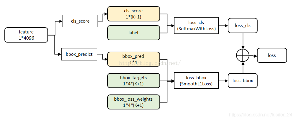
具体每个变量的意义还是看论文，写得很清楚。Ncls=256，Nreg~=2000，λ=10。
分类使用softmax回归，使用的是交叉熵损失函数，公式：

代码：

		rpn_data = self.RPN_anchor_target((rpn_cls_score.data, gt_boxes, im_info, num_boxes))
        # compute classification loss
        rpn_cls_score = rpn_cls_score_reshape.permute(0, 2, 3, 1).contiguous().view(batch_size, -1, 2)
        rpn_label = rpn_data[0].view(batch_size, -1)

        rpn_keep = Variable(rpn_label.view(-1).ne(-1).nonzero().view(-1))
        rpn_cls_score = torch.index_select(rpn_cls_score.view(-1,2), 0, rpn_keep)
        rpn_label = torch.index_select(rpn_label.view(-1), 0, rpn_keep.data)
        rpn_label = Variable(rpn_label.long())
        self.rpn_loss_cls = F.cross_entropy(rpn_cls_score, rpn_label)
        fg_cnt = torch.sum(rpn_label.data.ne(0))

边界框的线性回归损失函数。线性回归就是给定输入的特征向量X, 学习一组参数W, 使得经过线性回归后的值跟真实值Y（即GT）非常接近，即Y=WX。对于该问题，输入X是一张经过卷积获得的feature map，定义为Φ；同时还有训练传入的GT。

这里R用smooth L1损失函数。Lerg前面乘一个p*，说明只有正样本，即forground anchor对损失函数有贡献，bg anchor贡献为0。smooth L1是一个平滑的绝对值函数，公式如下：

只有在GT与需要回归框位置比较接近时，可以认为是线性变换。论文里是这么写的：

where x, y, w, and h denote the box’s center coordinates and its width and height. Variables x, xa, and
x∗ are for the predicted box, anchor box, and groundtruth box respectively (likewise for y, w, h).

代码如下：

# compute bbox regression loss
        rpn_bbox_inside_weights = Variable(rpn_bbox_inside_weights)
        rpn_bbox_outside_weights = Variable(rpn_bbox_outside_weights)
        rpn_bbox_targets = Variable(rpn_bbox_targets)
        self.rpn_loss_box = _smooth_l1_loss(rpn_bbox_pred, rpn_bbox_targets, rpn_bbox_inside_weights,
                                                        rpn_bbox_outside_weights, sigma=3, dim=[1,2,3])