【机器学习】--KNN

仅记录学习过程。

一句话介绍：

KNN是一种可用于分类和回归的方法。一般情况下用其进行分类任务。

KNN三要素：

1）模型，即对特征空间的划分；
2）距离度量，欧氏距离等；
3）分裂决策规则，即多数投票方法

特点：

KNN不具有显式的学习过程，实际上是利用训练集对特征空间进行划分，然后对新样本进行相邻K个最近样本的统计，并以多数类作为该样本的预测。

理论部分就不做阐述了，直接上代码

先来一段用线性模块来做回归模型的代码。

主要过程为：数据准备，建立模型，训练模型，测试数据。

from sklearn import datasets, linear_model # 引用 sklearn库，主要为了使用其中的线性回归模块
# 创建数据集，把数据写入到numpy数组
import numpy as np  # 引用numpy库，主要用来做科学计算
import matplotlib.pyplot as plt   # 引用matplotlib库，主要用来画图

# 创建数据，数据的内容为身高体重的关系。
data = np.array([[152,51],[156,53],[160,54],[164,55],
                 [168,57],[172,60],[176,62],[180,65],
                 [184,69],[188,72]])

# 打印出数组的大小
print(data.shape)
x,y = data[:,0].reshape(-1,1), data[:,1] #　得到特征和标签x和y
# TODO 1. 实例化一个线性回归的模型,并把这个模型命名为rege
regr = linear_model.LinearRegression()
# TODO 2. 在x,y上训练一个线性回归模型.如果训练顺利,则regr会存储训练完成之后的结果模型
regr.fit(x, y)
# TODO 3. 画出身高与体重之间的关系
plt.scatter(x, y, color='red')
# 画出已训练好的线条
plt.plot(x, regr.predict(x), color='blue')
# 画x,y轴的标题
plt.xlabel('height (cm)')
plt.ylabel('weight (kg)')
plt.show()

# 利用已经训练好的模型去预测身高为163的人的体重
print ("Standard weight for person with 163 is %.2f"% regr.predict([[163]]))

 

自己动手写KNN分类器：

from sklearn import datasets
from collections import Counter  # 为了做投票
from sklearn.model_selection import train_test_split
import numpy as np
# 导入iris数据
iris = datasets.load_iris()
X = iris.data
y = iris.target
X_train, X_test, y_train, y_test = train_test_split(X, y, random_state=2003)

def euc_dis(instance1, instance2):
    """
    计算两个样本instance1和instance2之间的欧式距离
    instance1: 第一个样本， array型
    instance2: 第二个样本， array型
    """
    # TODO
    dist = np.sqrt(sum((instance1 - instance2) ** 2))
    return dist

def knn_classify(X, y, testInstance, k):
    """
    给定一个测试数据testInstance, 通过KNN算法来预测它的标签。
    X: 训练数据的特征
    y: 训练数据的标签
    testInstance: 测试数据，这里假定一个测试数据 array型
    k: 选择多少个neighbors?
    """
    # TODO  返回testInstance的预测标签 = {0,1,2}
    distances = [euc_dis(x, testInstance) for x in X]
    kneighbors = np.argsort(distances)[:k]
    count = Counter(y[kneighbors])
    return count.most_common()[0][0]

# 预测结果。
predictions = [knn_classify(X_train, y_train, data, 3) for data in X_test]
correct = np.count_nonzero((predictions == y_test) == True)
print("Accuracy is: %.3f" % (correct / len(X_test)))

 

用sklearn中的模型实现KNN，并用2中方法实现交叉验证。

方法一：

import numpy as np
from sklearn import datasets
from sklearn.neighbors import KNeighborsClassifier
from sklearn.model_selection import KFold

# 加载iris数据集
iris = datasets.load_iris()
X = iris.data
y = iris.target
print(X.shape, y.shape)

# 定义我们想要搜索的k值，这里定义8个不同的值
ks = [1, 3, 5, 7, 9, 11, 13, 15]
kf = KFold(n_splits=5, random_state=2001, shuffle=True)

best_k = ks[0]
best_score = 0

for k in ks:
    curr_score = 0
    for train_index, valid_index in kf.split(X):
        # 每一折的训练以及计算准确率
        clf = KNeighborsClassifier(n_neighbors=k)
        clf.fit(X[train_index], y[train_index])
        curr_score += clf.score(X[valid_index], y[valid_index])
        avg_score = curr_score / 5
        if avg_score > best_score:
            best_k = k
            best_score = avg_score
    print("current best score is ：%.2f" % best_score, "best k :%d" % best_k)

print("after cross validation,the final best k is :%d" % best_k)

方法二：

from sklearn.model_selection import GridSearchCV
from sklearn import datasets
from sklearn.neighbors import KNeighborsClassifier

iris = datasets.load_iris()
X = iris.data
y = iris.target

# 设置需要搜索的k值，“n_neighbors”是sklearn中KNN中的参数
parameters = {'n_neighbors':[1,3,5,7,9,11,13,15]}
knn = KNeighborsClassifier()

clf = GridSearchCV(knn,parameters,cv=5)
clf.fit(X,y)

print("best score is :%2f"%clf.best_score_,"best param :",clf.best_params_)

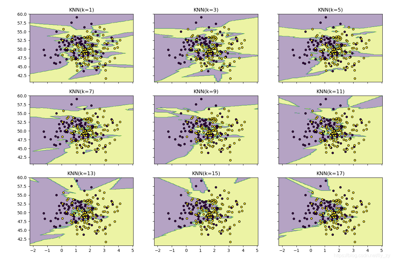
用不同的K值对数据进行学习，并实现可视化。

import matplotlib.pyplot as plt
import numpy as np
from itertools import product
from sklearn.neighbors import  KNeighborsClassifier

# 生成一些随机样本

n_point = 100
x1 = np.random.multivariate_normal([1,50],[[1,0],[0,10]],n_point)
x2 = np.random.multivariate_normal([2,50],[[1,0],[0,10]],n_point)
X = np.concatenate([x1,x2])
y = np.array([0]*n_point+[1]*n_point)
print(X.shape,y.shape)

# KNN模型的训练过程
clfs = []
neighbors = [1,3,5,7,9,11,13,15,17]
for i in range(len(neighbors)):
    clfs.append(KNeighborsClassifier(neighbors[i]).fit(X,y))

# 可视化结果
x_min,x_max = X[:,0].min()-1,X[:,0].max()+1     # 得到x轴的最大值和最小值，方便画图
y_min,y_max = X[:,1].min()-1,X[:,1].max()+1   # 得到y轴的最大最小值，并留一段距离，画出来的图形好看
xx,yy = np.meshgrid(np.arange(x_min,x_max,0.1),    # 生成网格图
                    np.arange(y_min,y_max,0.1))

f,axarr = plt.subplots(3,3,sharex='col',sharey='row',figsize=(15,12))

for idx,clf,tt in zip(product([0,1,2],[0,1,2]),clfs,
                      ['KNN(k=%d)'%k for k in neighbors]):
    z = clf.predict(np.c_[xx.ravel(),yy.ravel()])
    z = z.reshape(xx.shape)

    axarr[idx[0],idx[1]].contourf(xx,yy,z,alpha=0.4)
    axarr[idx[0], idx[1]].scatter(X[:,0],X[:,1],c=y,s=20,edgecolor='k')
    axarr[idx[0], idx[1]].set_title(tt)

plt.show()

输出为：