N-step Bootstrapping For Advantage Actor-Critic

by Xiaoxiao Wen, Yijie Zhang, Zhenyu Gao, Weitao Luo

1 Introduction and Motivation

In this project, we study n-step bootstrapping in actor critic methods [1], more specific, we would like to investigate, when using n-step bootstrapping for advantage actor critic (A2C), how different values of $n$ will affect the model performances, measured by different metrics, for example, convergence speed and stability (variance).

1.1 N-step bootstrapping

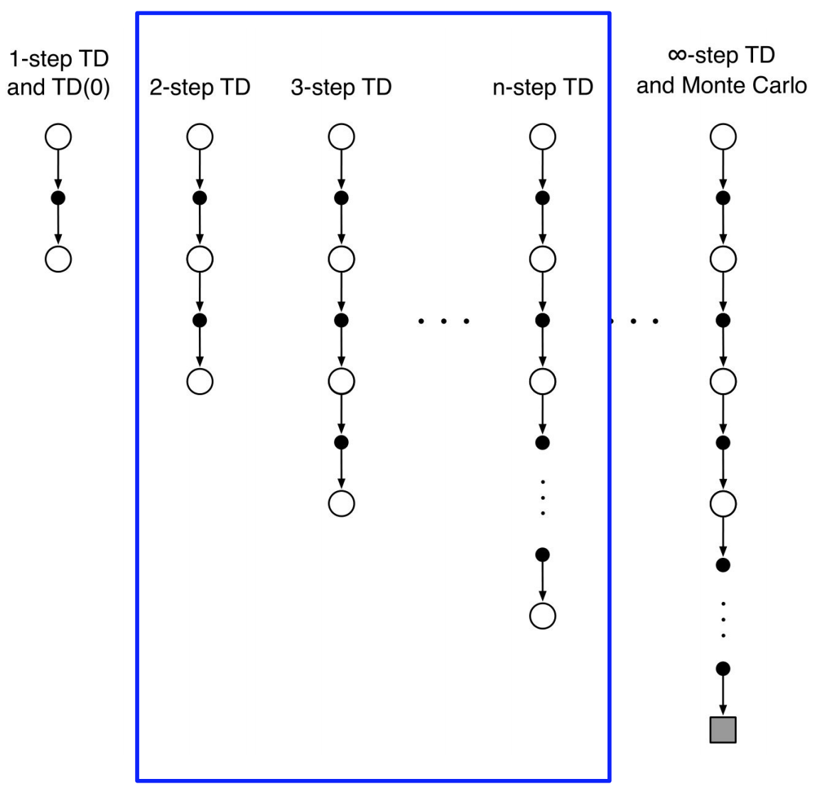
N-step bootstrapping [1], or TD(N) is a very important technique in Reinforcement Learning that performs update based on intermediate number of rewards. In this view, N-step bootstrapping unifies and generalizes the Monte Carlo (MC) methods and Temporal Difference (TD) methods. From one extreme, when $N=1$, it is equivalent to TD(1), from another extreme, when $N=\infty$, i.e., taking as many steps as possible until the end of the episode, it becomes MC. As a result, N-step bootstrapping also combines the advantages of Monte Carlo and 1-step TD. Compared to 1-step TD, n-step bootstrapping will converge faster because it bootstraps with more real information and it is freed from the “tyranny of the time step”. Compared to MC, the updates do not have to wait until the end of the episode and it is also more efficient and less variants. In general, when facing different problems / situations, with a suitable N, we could often achieve faster and more stable learning.

Figure1: Diagrams for n-step bootstrapping.

1.2 Advantage Actor Critic (A2C)

Actor-Critic algorithms are a power families of learning algorithms within the policy-based framework in Reinforcement Learning. It composes of actor, the policy that makes decision and critic, the value function that evaluates if it is a good decision. With the assistant from critic, the actor can usually achieves better performance, such as by reducing gradient variance in vanilla policy gradients. From the GAE paper [2], John Schulman has unified the framework for advantage estimation, between all the GAE variants, we picked A2C considering the amazing performance of A3C and it is a simplified version of A3C with equivalent performance.

In the following sections, we first explain the method of n-step Bootstrapping for A2C, which also includes 1-step and Monte-Carlo as mentioned above, and then briefly introduce the neural network architecture. Subsequently, we introduce the conducted experiments with their corresponding settings and finally we discuss the results and draw some conclusions.

2 Methods

n-step Bootstrapping for A2C

n-step A2C is an online algorithm that uses roll-outs of size n + 1 of the current policy to perform a policy improvement step. In order to train the policy-head, an approximation of the policy-gradient is computed for each state of the roll-out ${\left(x_{t+i},a_{t+i}\sim \pi \left(\cdot |x_{t+i};{\theta }_{\pi }\right),r_{t+i}\right)}_{i=0}^n$, expressed as
$${\nabla }_{{\theta }_{\pi }}\log \left(\pi \left(a_{t+i}|x_{t+i};{\theta }_{\pi }\right)\right)\left[{\hat{Q}}_i-V\left(x_{t+i};{\theta }_V\right)\right]$$
where ${\hat{Q}}_i$ is an estimation of the return ${\hat{Q}}_i={\sum }_{j=i}^{n-1}{\gamma }^{j-i}{r}_{t+j}+{\gamma }^{n-i}V\left(x_{t+n};{\theta }_V\right)$. The gradients $j=i$
are then added to obtain the cumulative gradient of the roll-out as
$$\sum _{i=0}^n{\nabla }_{{\theta }_{\pi }}\log \left(\pi \left(a_{t+i}|x_{t+i};{\theta }_{\pi }\right)\right)\left[{\hat{Q}}_i-V\left(x_{t+i};{\theta }_V\right)\right]$$
A2C trains the value-head by minimising the error between the estimated return and the value as
$$\sum _{i=0}^n{\left({\hat{Q}}_i-V\left(x_{t+i};{\theta }_V\right)\right)}^2$$

Therefore, the network parameters $\left({\theta }_{\pi },{\theta }_V\right)$ are updated after each roll-out as follows:
$$\begin{array}{l}{\theta }_{\pi }\leftarrow {\theta }_{\pi }+{\alpha }_{\pi }{\sum }_{i=0}^n{\nabla }_{{\theta }_{\pi }}\log \left(\pi \left(a_{t+i}|x_{t+i};{\theta }_{\pi }\right)\right)\left[{\hat{Q}}_i-V\left(x_{t+i};{\theta }_V\right)\right]\\ {\theta }_V\leftarrow {\theta }_V-{\alpha }_V{\sum }_{i=0}^n{\nabla }_{{\theta }_V}{\left[{\hat{Q}}_i-V\left(x_{t+i};{\theta }_V\right)\right]}^2\end{array}$$
where $\left({\alpha }_{\pi },{\alpha }_V\right)$ are learning rates are policy-head and value-head.

2.2 Network Architecture

Similar to the $Actor-criticexamplefrompytorch$ and $Floodsun{g}^{\prime }srepo$, we use simple and straightforward networks for both the actor function and the critic function.

2.2.1 Actor Network

The actor network consists of two fully connected layers which extract potential features from the input observations. To introduce non-linearity, the ReLU activations [3] are used upon these two layers. Then, the output is another fully connected layer which summarizes into one-dimensional continuous value.

2.2.2 Critic Network

The critic network shares the similar architecture with the actor network with the fully connected layers and the ReLU activations. However, depending on the environment, discrete or continuous action space, the final output is distinct. For discrete action space, the $\log$ Softmax is used to compute the distribution of the available discrete actions. For continuous action space, we instead output a mean and a standard deviation for the univariate Gaussian distribution, which we later use to sample continuous actions.

3 Experiments

All our code can be see in Github.

Reinforcement Learning Reproducibility Lab

3.1 Environments

For this project, our main goal is to compare the performance of the n-step bootstrapping variation of A2C with its Monte-Carlo and 1-step variations in a straightforward manner. Therefore, we do not seek to deliver an ultimate agent that can solve some complicated fancy games or park your car.

The experiments are designed with classical control problems, i.e. InvertedPendulum, CartPole, Acrobot, MountainCar etc. For the sake of convenience in terms of implementation, we use the off-the-shelf environments provided by $OpenA{I}^{\prime }sGymlibrary$. Under the category $\text{Classical Control}$, we picked out two discrete environments: $\text{CartPole-v0}$ and $\text{Acrobot-v1}$.

The $\text{CartPole-v0}$ environment contains a pole attached by a an un-actuated joint to a cart in a 2D plane. The cart moves left/right along a frictionless track. The goal is to balance the poll staying upright by indirectly influencing the velocity of the cart. There are 4 continuous observations of this environment, consisting of the $\text{Cart Position}$, $\text{Cart Velocity}$, $\text{Pole Angle}$ and $\text{Pole Velocity At Tip}$ within their corresponding range. The available actions consist of two discrete actions $\text{Push Left}$ and $\text{Push Right}$, which increases the $\text{Cart Velocity}$ by an unknown amount in the corresponding direction. At starting state, all the observations are initialized with a small uniform random value. The termination of each episode is defined by the pole angle’s or the cart position’s exceeding a certain threshold, or when the episode length exceeds 200 steps. The reward is 1 for every step taken in each episode, indicating the durability of the stabilization by the agent. You can see it in the Figure 2 (Form “Using Bayesian Optimization for Reinforcement Learning”).

Figure2: Cartpole.

The $\text{Pendulum-v0}$ environment contains a pendulum, or in other words, a link connected to an actuated joint in a 2D plane. The pendulum can spin frictionlessly. The goal is to keep the pendulum upright by applying a continuous torque on the joint. There are 3 continuous observations of this environment, consisting of the $\cos$ and $\sin$ values of the $\text{Pendulum Angle}$ respectively and the $\text{Angular Velocity}$ of the pendulum. The available action is a continuous action $\text{Apply Torque}$. At starting state, the pendulum is initiated at a random angle and a random angular velocity. The environment is terminated when the episode length exceeds 200 steps. The reward is computed according to a function of the angle, angular velocity and the torque, which ranges from $-16$ to $0$, so the goal can be explained as to remain at zero angle, with the least angular velocity and the least torque, indicating the speed and the quality of the stabilization by the agent. You can see it in Figure 3 (From “Solving Reinforcement Learning Classic Control Problems | OpenAIGym”).

Figure3: Pendulum

3.2 Settings

The hyperparameter settings are trivial for the actor and critic networks. In the aforementioned fully connected layers, we use a hidden size of 64 nodes, which we found empirically. Furthermore, the discount rate $\gamma$ is set to 0.99.

In order to evaluate how different $n$ will affect the performances, we need to conduct experiments and investigate the model behaviors in different learning stages.

To make the comparison objective and accurate, instead of fixing the number of training episodes, we fix the total number of $10000$ training steps. More specific, for training, each agent will interact and learn in the environments for $100$ steps according to their updating schemes strictly (n-steps, TD or MC). For example, if in a training cycle, the MC agent starts in time-step 14 and after 86 steps (totally 100 steps) the episode still continues, the MC agent will not receive any updates. Then, for evaluation, we run the agent in the exact environments as in training for 50 episodes and store the total rewards per episode. With this data, the learning behavior and model performance of each agent can be represented and compared scientifically in terms of mean and standard deviation per evaluation step and, furthermore, the mean and variance could be used to show the effectiveness and stability of learning accordingly.

To fully cover MC, TD and n-step bootstrapping, we chose and tested 6 different $n$ given the different termination conditions of two environments, which ranges from 1-step to max-step (or equivalently Monte Carlo). Finally, to decrease the effect of randomness, three different random seeds are tested and the experiment settings are shown in Table 1.

• Training: each agent will gain experience in the environment for every $100$ steps and learn (or update their networks) according to their schemes.
• Evaluation: after very $100$ training steps, each agents will be tested in the same environments and play for $50$ episodes. There will be no learning in this stage and the rewards will be stored.

Table1: Hyperparameter settings of the experiments.

Environment	Train Steps	Eval Interval	Eval steps	Random Seeds	Steps Roll-out
CartPole-v0	10000	100	50	[42, 36, 15]	[1, 10, 40, 80, 150, 200]
Pendulum-v0	10000	100	50	[42, 36, 15]	[1, 10, 40, 80, 150, 200]

4 Results

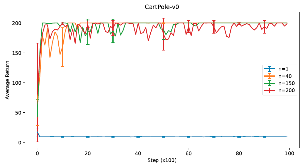
The results are shown in Figure 4 - Figure 7, where for better visualization and distinction, only two n-step variations are selected.

4.1 CartPole

As shown in Figure 4, generally, except for 1-step TD, all the variations converge finally to the expected average return of $200$. The 1-step TD fails to learn and achieve an average reward of around 10, which is possibly because of the complexity of the environment, where the bias in 1-step learning is too large and the learning diverges. It can also be observed that, with increasing $n$, the variance increases, which also aligns with the fact that for Monte-Carlo methods compared with 1-step TD methods, the bias is low but the variance is high, and vice versa.

Figure 4: Results for CartPole-v0.

Furthermore, observing the truncated results for 3000 steps in Figure 5, we can see that because of the relatively higher biases for smaller $n$'s (40), the convergences are significantly slower. While for $n=150$ and $n=200$, the convergence is fast.

Figure 5: Results for CartPole-v0.

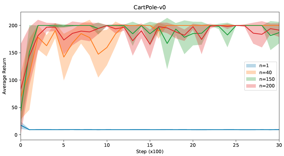
To summarize, by taking into consideration both the convergence stability and the convergence speed, a relatively good performance is observed for $n=40$.

4.2 Pendulum

As shown in Figure 6, in general, the performance is not as good as the CartPole case, and convergence is hardly achieved. For $n=40$, it is obvious that the learning curve tends to increase and converge, but for the other curves, given the high variance, no similar conclusions can be made. Nonetheless, the pattern with bias and variance trade-off w.r.t. $n$ can still be observed, as the standard deviations for smaller $n$'s (1, 40) are relatively higher than those for larger $n$'s (150, 200).

Figure 6: Results for Pendulum-v0.

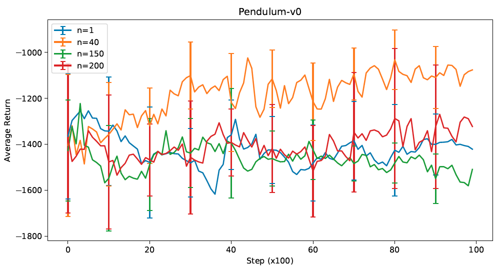
On the other hand, by observing the truncated results in Figure 7, it can be seen that for $n=40$, there tends to be a faster convergence compared to the others.

Figure 7: Results for Pendulum-v0.

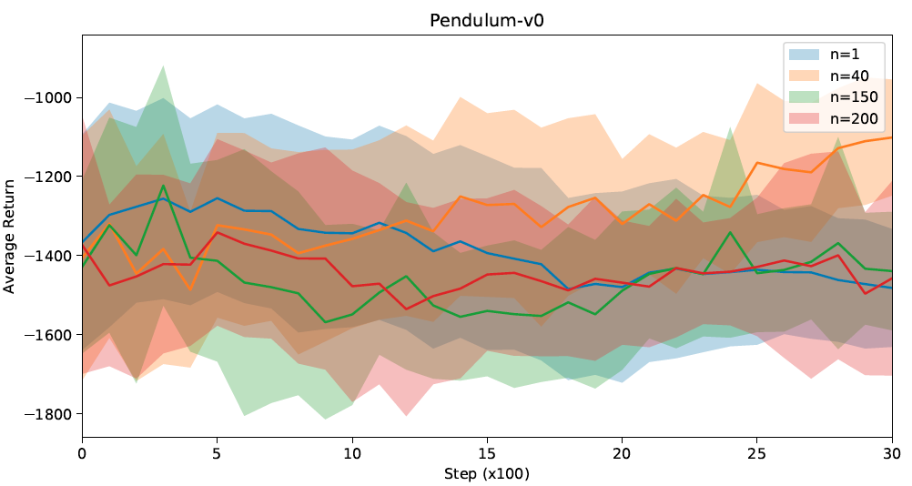
To summarize, $n=40$ would be the preferable choice for this environment.

Conclusion

In this project, we investigate how different n for n-step bootstrapping could affect the learning behaviors of the A2C agent. We show that when using n=1, i.e., the TD method, the A2C agents are seldom capable of learning for both the CartPole and Pendulum environments. While using MC, for the CartPole environment, the A2C agents are capable of learning with faster convergence but show a more volatile and unstable behaviors. However, for the Pendulum environment, convergence is not observed and future investigations need to be done. After the experiments, in general, we show that n-step bootstrapping achieves a relatively better performance in terms of convergence stability and the convergence speed compared to 1-step TD and MC by compensating between bias and variance. Hence, choosing an appropriate intermediate n could be vital for different application or problems in Reinforcement Learning.

References

[1] Sutton, Richard S., and Andrew G. Barto. Reinforcement learning: An introduction. MIT press, 2018.
[2] Schulman, John, et al. “High-dimensional continuous control using generalized advantage estimation.” arXiv preprint arXiv:1506.02438 (2015).
[3] Agarap, Abien Fred. “Deep learning using rectified linear units (relu).” arXiv preprint arXiv:1803.08375 (2018).