RC circuit

最新推荐文章于 2022-07-30 18:31:24 发布

原创最新推荐文章于 2022-07-30 18:31:24 发布 · 749 阅读

0 ·

CC 4.0 BY-SA版权

文章标签：

#components #combinations #signal #function #filter #output

本文深入探讨了RC电路的基本原理，包括其组成、行为特征及其在不同情况下的应用。文章重点介绍了RC电路作为低通和高通滤波器的功能，并详细解释了其在频率域和时间域的表现，以及如何通过拉普拉斯变换求解电路行为。

摘要生成于 C知道，由 DeepSeek-R1 满血版支持，前往体验 >

Introduction

There are three basic, linear analog circuit components: the resistor (R), capacitor (C) and inductor (L). These may be combined in four important combinations: the RC circuit, the RL circuit, the LC circuit and the RLC circuit with the abbreviations indicating which components are used. These circuits, between them, exhibit a large number of important types of behaviour that are fundamental to much of analog electronics. In particular, they are able to act as passive filters. This article considers the RC circuit, in both series and parallel as shown

Natural response

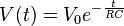
The simplest RC circuit is a capacitor and a resistor in series. When a circuit composes of only a charged capacitor and a resistor, then the capacitor would discharge its energy into the resistor. This voltage across the capacitor over time could be found through KCL, where the current coming out of the capacitor must equal the current going through the resistor. This results in the linear differential equation

$C/frac{dV}{dt} + /frac{V}{R}=0$ .

When solved, it results in the exponential decay function

$V(t)=V_0 e^{-/frac{t}{RC}}$

Complex impedance

The equivalent resistance of a capacitor increases in relation to the amount of charge stored on the capacitor. If a capacitor is subjected to an alternating current voltage source, then the voltage of the capacitor would flip to the frequency of the AC voltage source. The faster the voltage of the AC voltage source flips, the less time charge would allowed to be stored on the capacitor, therefore reducing the capacitor's equivalent resistance. This explains the inverse relationship the equivalent resistance of a capacitor has with the frequency of the voltage source.

The resistance, also known as the complex impedance, Z_C (in ohms) of a capacitor with capacitance C (in farads) is

$Z_C = /frac{1}{sC}$

The angular frequency s is, in general, a complex number,

$s / = / /sigma + j /omega$

where

j represents the imaginary unit:

j 2 = - 1

$/sigma /$ is the exponential decay constant (in radians per second), and
$/omega /$ is the sinusoidal angular frequency (also in radians per second).

Sinusoidal steady state

Sinusoidal steady state is a special case in which the input voltage consists of a pure sinusoid (with no exponential decay). As a result,

$/sigma / = / 0$

and the evaluation of s becomes

$s / = / j /omega$

Series circuit

Series RC circuit

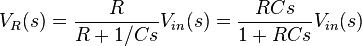
By viewing the circuit as a voltage divider, the voltage across the capacitor is:

$V_C(s) = /frac{1/Cs}{R + 1/Cs}V_{in}(s) = /frac{1}{1 + RCs}V_{in}(s)$

and the voltage across the resistor is:

$V_R(s) = /frac{R}{R + 1/ Cs}V_{in}(s) = /frac{ RCs}{1 + RCs}V_{in}(s)$ .

Transfer functions

The transfer function for the capacitor is

$H_C(s) = { V_C(s) /over V_{in}(s) } = { 1 /over 1 + RCs }$ .

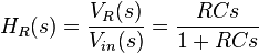
Similarly, the transfer function for the resistor is

$H_R(s) = { V_R(s) /over V_{in}(s) } = { RCs /over 1 + RCs }$ .

Poles and zeros

Both transfer functions have a single pole located at

$s = - {1 /over RC }$ .

In addition, the transfer function for the resistor has a zero located at the origin.

Gain and phase angle

The magnitude of the gains across the two components are:

$G_C = | H_C(j /omega) | = /left|/frac{V_C(j /omega)}{V_{in}(j /omega)}/right| = /frac{1}{/sqrt{1 + /left(/omega RC/right)^2}}$

and

$G_R = | H_R(j /omega) | = /left|/frac{V_R(j /omega)}{V_{in}(j /omega)}/right| = /frac{/omega RC}{/sqrt{1 + /left(/omega RC/right)^2}}$ ,

and the phase angles are:

$/phi_C = /angle H_C(j /omega) = /tan^{-1}/left(-/omega RC/right)$

and

$/phi_R = /angle H_R(j /omega) = /tan^{-1}/left(/frac{1}{/omega RC}/right)$ .

These expressions together may be substituted into the usual expression for the phasor representing the output:

$V_C / = / G_{C}V_{in} e^{j/phi_C}$

$V_R / = / G_{R}V_{in} e^{j/phi_R}$ .

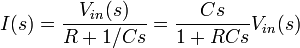
Current

The current in the circuit is the same everywhere since the circuit is in series:

$I(s) = /frac{V_{in}(s) }{R+1/ Cs} = { Cs /over 1 + RCs } V_{in}(s)$

Impulse response

The impulse response for each voltage is the inverse Laplace transform of the corresponding transfer function. It represents the response of the circuit to an input voltage consisting of an impulse or Dirac delta function.

The impulse response for the capacitor voltage is

$h_C(t) = {1 /over RC} e^{-t / RC} u(t) = { 1 /over /tau} e^{-t / /tau} u(t)$

where u(t) is the Heaviside step function and

$/tau / = / RC$

is the time constant.

Similarly, the impulse response for the resistor voltage is

$h_R(t) = /delta (t) - {1 /over RC} e^{-t / RC} u(t) = /delta (t) - { 1 /over /tau} e^{-t / /tau} u(t)$

where δ(t) is the Dirac delta function

Frequency-domain considerations

These are frequency domain expressions. Analysis of them will show which frequencies the circuits (or filters) pass and reject. This analysis rests on a consideration of what happens to these gains as the frequency becomes very large and very small.

As $/omega /to /infty$ :

$G_C /to 0$

$G_R /to 1$ .

As $/omega /to 0$ :

$G_C /to 1$

$G_R /to 0$ .

This shows that, if the output is taken across the capacitor, high frequencies are attenuated (rejected) and low frequencies are passed. Thus, the circuit behaves as a low-pass filter. If, though, the output is taken across the resistor, high frequencies are passed and low frequencies are rejected. In this configuration, the circuit behaves as a high-pass filter.

The range of frequencies that the filter passes is called its bandwidth. The point at which the filter attenuates the signal to half its unfiltered power is termed its cutoff frequency. This requires that the gain of the circuit be reduced to

$G_C = G_R = /frac{1}{/sqrt{2}}$ .

Solving the above equation yields

$/omega_{c} = /frac{1}{RC} / /mathrm{rad/s}$

$f_c = /frac{1}{2/pi RC} / /mathrm{Hz}$

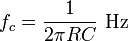
which is the frequency that the filter will attenuate to half its original power.

Clearly, the phases also depend on frequency, although this effect is less interesting generally than the gain variations.

As $/omega /to 0$ :

$/phi_C /to 0$

$/phi_R /to 90^{/circ} = /pi/2^{c}$ .

As $/omega /to /infty$ :

$/phi_C /to -90^{/circ} = -/pi/2^{c}$

$/phi_R /to 0$

So at DC (0 Hz), the capacitor voltage is in phase with the signal voltage while the resistor voltage leads it by 90°. As frequency increases, the capacitor voltage comes to have a 90° lag relative to the signal and the resistor voltage comes to be in-phase with the signal.

Time-domain considerations

This section relies on knowledge of e , the natural logarithmic constant.

The most straightforward way to derive the time domain behaviour is to use the Laplace transforms of the expressions for $V C$ and $V R$ given above. This effectively transforms $j/omega /to s$ . Assuming a step input (i.e. $V i n = 0$ before $t = 0$ and then $V i n = V$ afterwards):

$V_{in}(s) = V/frac{1}{s}$

$V_C(s) = V/frac{1}{1 + sRC}/frac{1}{s}$

and

$V_R(s) = V/frac{sRC}{1 + sRC}/frac{1}{s}$ .

Capacitor voltage step-response.

Resistor voltage step-response.

Partial fractions expansions and the inverse Laplace transform yield:

$/,/!V_C(t) = V/left(1 - e^{-t/RC}/right)$

$/,/!V_R(t) = Ve^{-t/RC}$ .

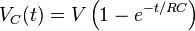
These equations are for calculating the voltage across the capacitor and resistor respectively while the capacitor is charging; for discharging, the equations are vice-versa. These equations can be rewritten in terms of charge and current using the relationships C=Q/V and V=IR (see Ohm's law).

Thus, the voltage across the capacitor tends towards V as time passes, while the voltage across the resistor tends towards 0, as shown in the figures. This is in keeping with the intuitive point that the capacitor will be charging from the supply voltage as time passes, and will eventually be fully charged and form an open circuit.

These equations show that a series RC circuit has a time constant, usually denoted $τ = R C$ being the time it takes the voltage across the component to either rise (across C) or fall (across R) to within $1 / e$ of its final value. That is, $τ$ is the time it takes $V C$ to reach $V (1 - 1 / e)$ and $V R$ to reach $V (1 / e)$ .

The rate of change is a fractional $/left(1 - /frac{1}{e}/right)$ per $τ$ . Thus, in going from $t = N τ$ to $t = (N + 1)τ$ , the voltage will have moved about 63.2 % of the way from its level at $t = N τ$ toward its final value. So C will be charged to about 63.2 % after $τ$ , and essentially fully charged (99.3 %) after about $5τ$ . When the voltage source is replaced with a short-circuit, with C fully charged, the voltage across C drops exponentially with t from $V$ towards 0. C will be discharged to about 36.8 % after $τ$ , and essentially fully discharged (0.7 %) after about $5τ$ . Note that the current, $I$ , in the circuit behaves as the voltage across R does, via Ohm's Law.

These results may also be derived by solving the differential equations describing the circuit:

$/frac{V_{in} - V_C}{R} = C/frac{dV_C}{dt}$

and

$/,/!V_R = V_{in} - V_C$ .

The first equation is solved by using an integrating factor and the second follows easily; the solutions are exactly the same as those obtained via Laplace transforms.