Lesson 07 for Plotting in R for Biologists

作者简介

taoyan：R语言中文社区特约作家，伪码农，R语言爱好者，爱开源。

个人博客: https://ytlogos.github.io/

前文传送门：

R语言可视化学习笔记之相关矩阵可视化包ggcorrplot

R语言学习笔记之相关性矩阵分析及其可视化

ggplot2学习笔记系列之利用ggplot2绘制误差棒及显著性标记

ggplot2学习笔记系列之主题（theme）设置

用circlize包绘制circos-plot

利用gganimate可视化R-Ladies发展情况

一篇关于国旗与奥运会奖牌的可视化笔记

利用ggseqlogo绘制seqlogo图

R语言data manipulation学习笔记之创建变量、重命名、数据融合

R语言data manipulation学习笔记之subset data

R语言可视化学习笔记之gganimate包

创建属于自己的调色板

Lesson 01 for Plotting in R for Biologists

Lesson 02&03 for Plotting in R for Biologists

Lesson 04 for Plotting in R for Biologists

Lesson 05 for Plotting in R for Biologists

Lesson 06 for Plotting in R for Biologists

这节课主要两个知识点，一个是图形分面，一个是图形嵌入。

数据加载及清洗

library(tidyverse)

theme_set(theme_gray())

my_data <- read.csv("variants_from_assembly.bed", sep = "\t", quote = '', stringsAsFactors = TRUE, header = FALSE)

names(my_data) <- c("chrom","start","stop","name","size","strand","type","ref.dist","query.dist")

head(my_data)

    

##   chrom     start      stop name size strand      type ref.dist query.dist

## 1     6 103832058 103832059  SV1  185      + Insertion        0        185

## 2     6 102958468 102958469  SV2  317      + Insertion      -14        303

## 3     6 102741692 102741693  SV3  130      +  Deletion      130          0

## 4     6 102283759 102283760  SV4 1271      + Insertion      -12       1259

## 5     6 101194032 101194033  SV5 2864      + Insertion      -13       2851

## 6     6 101056644 101056645  SV6  265      + Insertion        0        265

    

my_data <- my_data[my_data$chrom %in% c(seq(1:22), "X","Y"), ]

my_data$chrom <- factor(gsub("chr", "",my_data$chrom), levels = c(seq(1:22),"X","Y"))

my_data$type <- factor(my_data$type, levels = c("Insertion","Deletion","Expansion","Contraction"))

   

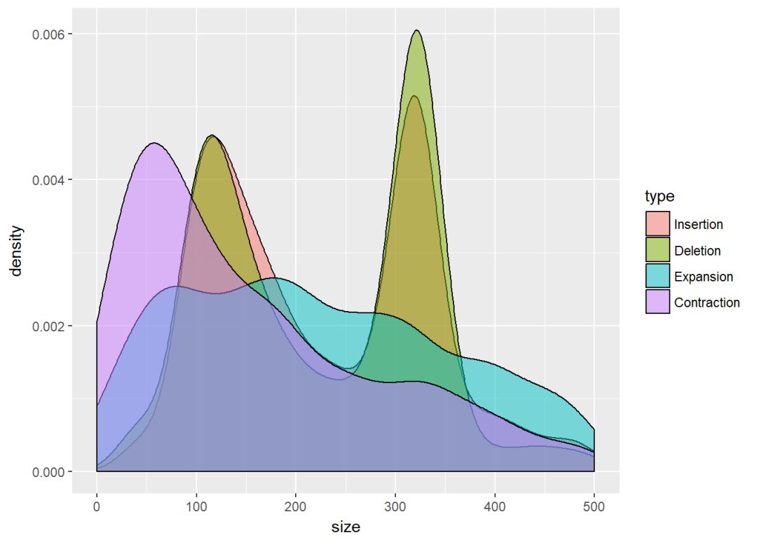
可视化&分面

ggplot(my_data, aes(x=size, fill=type))+geom_density(alpha=0.5)+xlim(0,500)

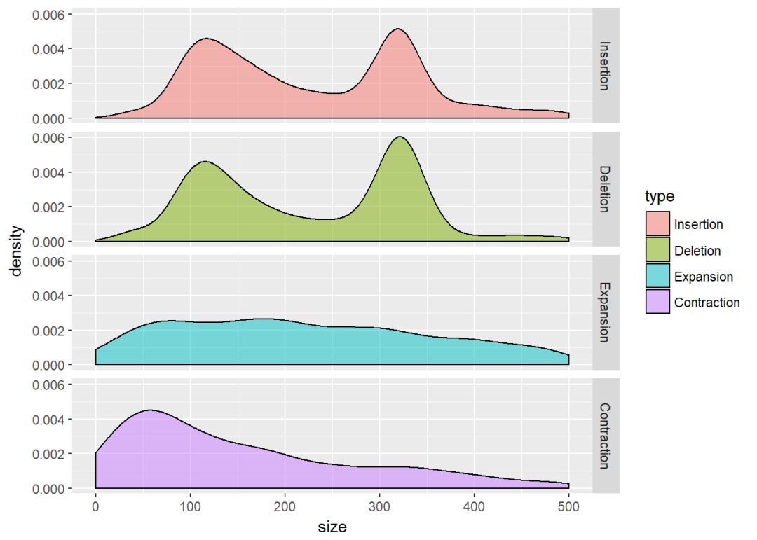
ggplot(my_data, aes(x=size, fill=type))+geom_density(alpha=0.5)+xlim(0,500)+facet_grid(type~.)

ggplot(my_data, aes(x=size, fill=type))+geom_density(alpha=0.5)+xlim(0,500)+facet_grid(.~type)

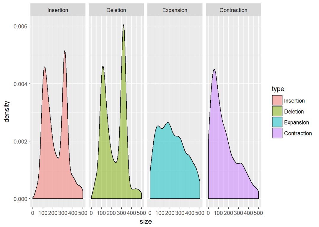
分面的规则语法是：  

plot+facet_grid(rows~columns)

比如下面的图按染色体为行、type为列进行分面

ggplot(my_data, aes(x=size, fill=type))+geom_density()+xlim(0,500)+facet_grid(chrom~type)

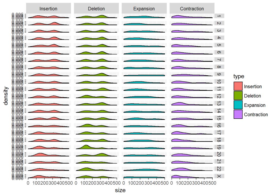
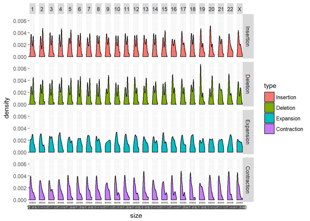
#也可以反过来

ggplot(my_data, aes(x=size, fill=type))+geom_density()+xlim(0,500)+facet_grid(type~chrom)

  

可以根据自己的喜好以及数据的分布进行分面，有的时候数据不是很适合分面操作，需要慎重，不然越分越乱，无法直观地展示数据。

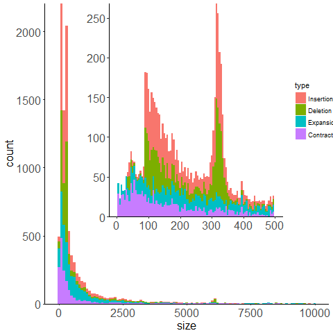
图形嵌入

#先设置主题

theme_set(theme_gray()+

theme(

axis.line = element_line(size=0.5),

panel.background = element_rect(fill=NA, size = rel(20)),

panel.grid.minor = element_line(colour = NA),

axis.text = element_text(size = 16),

axis.title = element_text(size = 16)

)

)

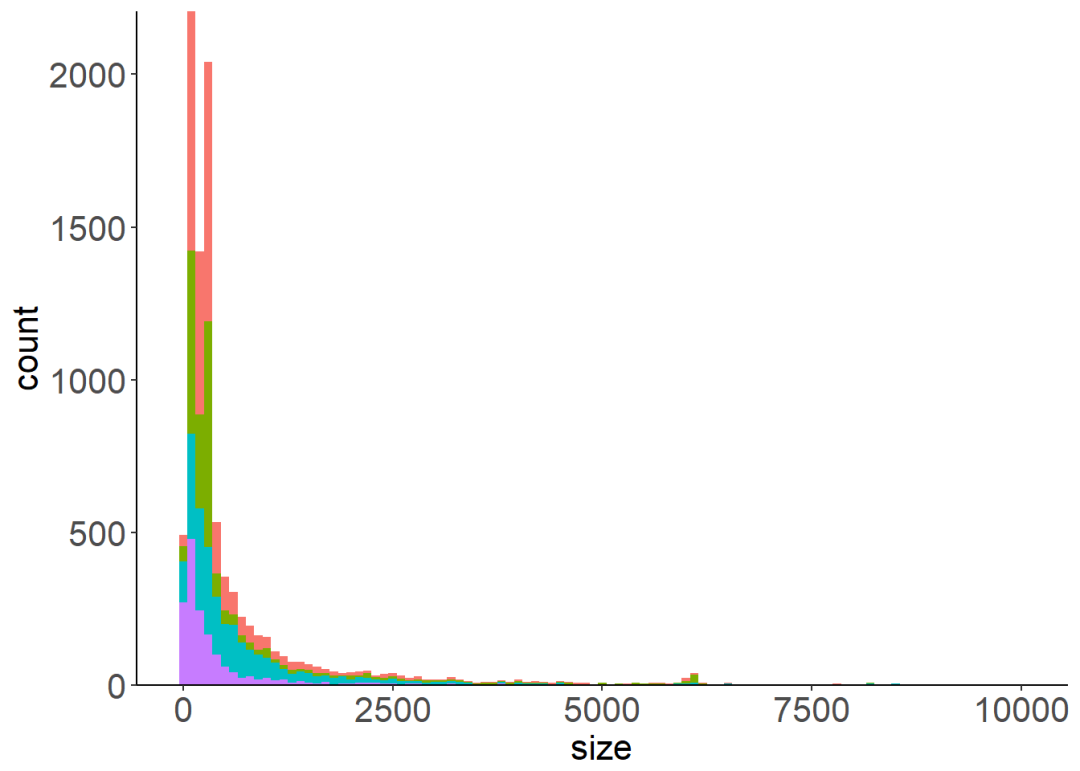
big_plot <- ggplot(my_data, aes(x=size, fill=type))+

geom_bar(binwidth = 100)+

guides(fill=FALSE)+

scale_y_continuous(expand = c(0,0))

big_plot

  

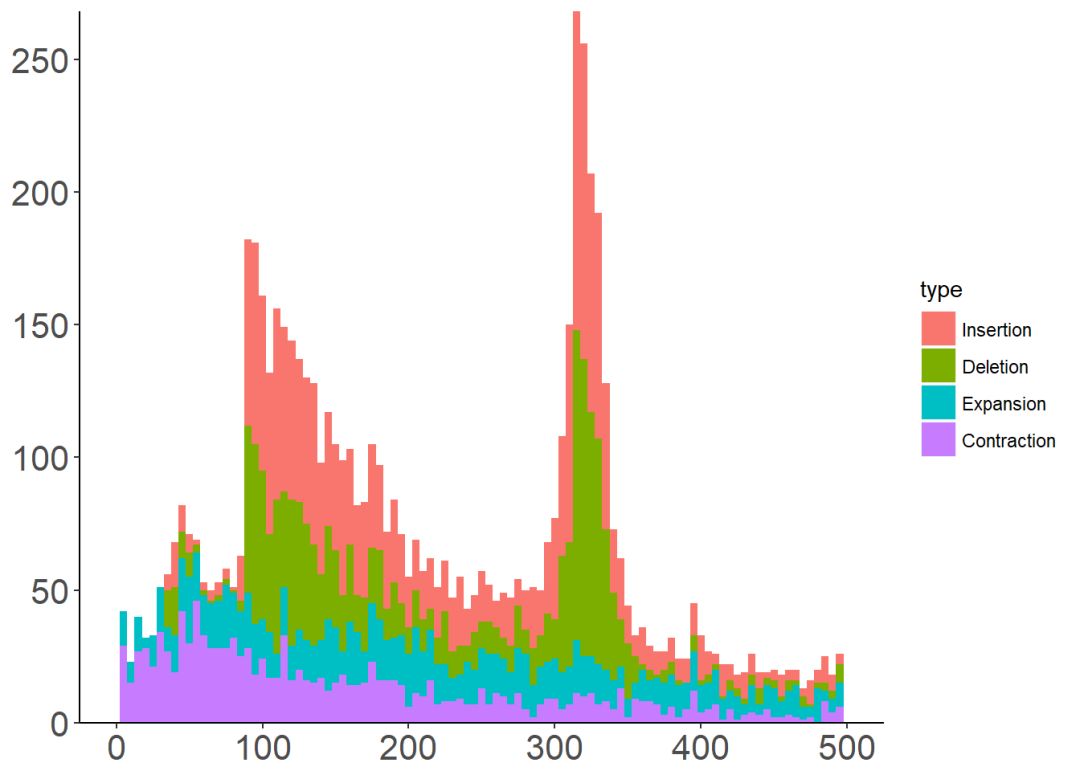
small_plot <- ggplot(my_data, aes(x=size, fill=type))+

geom_bar(binwidth = 5)+

xlim(0, 500)+

theme(axis.title = element_blank())+

scale_y_continuous(expand = c(0,0))

small_plot

图形嵌入需要使用包grid

library(grid)

#构造画布，这一步需要不断调整位置

vp <- viewport(width = 0.8, height = 0.7, x=0.65, y=0.65)#分别设置需要嵌入的图形的宽度、高度以及坐标位置

png("insert_plot.png")

print(big_plot)

print(small_plot, vp = vp)

dev.off()

SessionInfo

sessionInfo()

## R version 3.4.3 (2017-11-30)

## Platform: x86_64-w64-mingw32/x64 (64-bit)

## Running under: Windows 10 x64 (build 16299)

##

## Matrix products: default

##

## locale:

## [1] LC_COLLATE=Chinese (Simplified)_China.936

## [2] LC_CTYPE=Chinese (Simplified)_China.936  

## [3] LC_MONETARY=Chinese (Simplified)_China.936

## [4] LC_NUMERIC=C                              

## [5] LC_TIME=Chinese (Simplified)_China.936    

##

## attached base packages:

## [1] grid      stats     graphics  grDevices utils     datasets  methods  

## [8] base    

##

## other attached packages:

## [1] forcats_0.2.0      stringr_1.2.0      dplyr_0.7.4      

## [4] purrr_0.2.4        readr_1.1.1        tidyr_0.7.2      

## [7] tibble_1.4.2       ggplot2_2.2.1.9000 tidyverse_1.2.1  

##

## loaded via a namespace (and not attached):

##  [1] Rcpp_0.12.15      cellranger_1.1.0  pillar_1.1.0    

##  [4] compiler_3.4.3    plyr_1.8.4        bindr_0.1        

##  [7] tools_3.4.3       digest_0.6.15     lubridate_1.7.1  

## [10] jsonlite_1.5      evaluate_0.10.1   nlme_3.1-131    

## [13] gtable_0.2.0      lattice_0.20-35   pkgconfig_2.0.1  

## [16] rlang_0.1.6       psych_1.7.8       cli_1.0.0        

## [19] rstudioapi_0.7    yaml_2.1.16       parallel_3.4.3  

## [22] haven_1.1.1       bindrcpp_0.2      xml2_1.2.0      

## [25] httr_1.3.1        knitr_1.19        hms_0.4.1        

## [28] rprojroot_1.3-2   glue_1.2.0        R6_2.2.2        

## [31] readxl_1.0.0      foreign_0.8-69    rmarkdown_1.8    

## [34] modelr_0.1.1      reshape2_1.4.3    magrittr_1.5    

## [37] backports_1.1.2   scales_0.5.0.9000 htmltools_0.3.6  

## [40] rvest_0.3.2       assertthat_0.2.0  mnormt_1.5-5    

## [43] colorspace_1.3-2  labeling_0.3      stringi_1.1.6    

## [46] lazyeval_0.2.1    munsell_0.4.3     broom_0.4.3      

## [49] crayon_1.3.4

　往期精彩内容整理合集　

2017年R语言发展报告（国内）

精心整理 | R语言中文社区历史文章合集（作者篇）

公众号后台回复关键字即可学习

回复 R                  R语言快速入门及数据挖掘 
回复 Kaggle案例  Kaggle十大案例精讲（连载中）
回复 文本挖掘      手把手教你做文本挖掘
回复 可视化          R语言可视化在商务场景中的应用 
回复 大数据         大数据系列免费视频教程 
回复 量化投资      张丹教你如何用R语言量化投资 
回复 用户画像      京东大数据，揭秘用户画像
回复 数据挖掘     常用数据挖掘算法原理解释与应用
回复 机器学习     人工智能系列之机器学习与实践
回复 爬虫            R语言爬虫实战案例分享