Pytorch学习（6）-神经网络工具箱nn

最新推荐文章于 2025-03-10 13:58:50 发布

nonono吧

最新推荐文章于 2025-03-10 13:58:50 发布

阅读量583

点赞数 1

分类专栏：强化学习——Pytorch

本文链接：https://blog.youkuaiyun.com/ileopard/article/details/104145987

版权

强化学习——Pytorch 专栏收录该内容

8 篇文章

订阅专栏

nn模块是构建于autograd之上的神经网络模块。(autograd实现了自动微分系统)

1.1、nn.Module

由于使用autograd可实现深度学习模型，但是其抽象程度较低，用来实现深度学习模型，则需要编写的代码量极大。

因此torch.nn产生了，其是专门为深度学习设计的模块。torch.nn的核心数据结构是Module，它是一个抽象的概念，既可以表示神经网络中的某个层(layer)，也可以表示一个包含很多层的神经网络。

在实际使用中，通常是继承nn.Module，攥写自己的网络/层。

下面先来看看如何用nn.Module实现自己的全连接层。全连接层，又名仿射层，输出y和输入x满足y = Wx + b，W和b是可学习的参数。

全连接层的实现需要注意：

自定义层Linear必须继承nn.Module，并且在其构造函数中需调用nn.Module的构造函数，即super(Linear, self).__init__()或nn.Module.__init__(self)。
在构造函数__init__中必须自己定义可学习的参数，并封装成Parameter，如在下面例子里把w和b封装成Parameter。Parameter是一种特殊的Variable，但其默认需要求导(requires_grad=True)。
forward函数实现前向传播过程，其输入可以是一个或多个variable，对x的任何操作也必须是variable支持的操作
无需写反向传播函数，因其前向传播都是对variable进行操作，nn.Module能够利用autograd自动实现反向传播，这一点比Function简单许多。
使用时，直观上可将layer看成数学概念中的函数，调用layer(input)即可得到input对应的结果。它等价于layers.__call__(input)，在__call__函数中，主要调用的是layer.forward(x)。所以在实际使用中应尽量使用layer(x)而不是使用layer.forward(x)。
Module中的可学习参数可以通过named_parameters()或者parameter()返回迭代器，前者会给每个parameter附上名字，使其更具有辨识度。

class Linear(nn.Module):  # 继承nn.Module
    def __init__(self, in_features, out_features):
        super(Linear, self).__init__()  # 等价于nn.Module.__init__(self)
        self.w = nn.Parameter(t.randn(in_features, out_features))
        self.b = nn.Parameter(t.randn(out_features))

    def forward(self, x):
        x = x.mm(self.w)
        return x + self.b.expand_as(x)


layer = Linear(4, 3)
input = V(t.randn(2, 4))
output = layer(input)
print(output)

for name, parameter in layer.named_parameters():
    print(name, parameter)  # w和b
# -----------------------------------------------
tensor([[ 1.1202,  2.3926, -2.0179],
        [ 0.5567,  1.1519,  0.2462]], grad_fn=<AddBackward0>)
w Parameter containing:
tensor([[-0.9790, -0.3613, -0.2963],
        [ 0.7113,  0.0377,  0.4925],
        [-1.0212, -0.6085,  0.3077],
        [ 0.9080, -0.0354,  1.3085]], requires_grad=True)
b Parameter containing:
tensor([ 0.2244,  1.0853, -0.0439], requires_grad=True)
# -------------------------------------------------------------

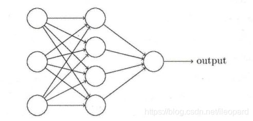
多层感知机的网络结果如下图所示，它由两个全连接层组成，采用sigmoid函数作为激活函数(图中没有画出)。

实现起来也很简单，如下代码，但需要注意两点：

构造函数__init__中，可利用前面自定义的Linear层(module）作为当前module对象的一个子module，它的可学习参数，也会成为当前module的可学习参数。
在前向传播函数中，将输入变量都命名成x，是为了能让Pytorch回收一些中间层的输出，从而节省内存。但并不是所有的中间结果都会被回收，有些variable虽然名字被覆盖，但其在反向传播时仍需要用到，此时Pytorch的内存回收模块将通过检查引用计数，不会回收则不复内存。

module中parameter的全局命名规范如下：

Parameter直接命名。例如self.param_name=nn.Parameter(t.randn(3, 4))，命名为param_name。
子module中的parameter，会在其名字之前加上当前module的名字。例如self.sub_module=SubModel()，SubModel中有个parameter名字也叫做param_name，那么二者拼接而成的parameter name就是sub_module.param_name。

class Linear(nn.Module):  # 继承nn.Module
    def __init__(self, in_features, out_features):
        super(Linear, self).__init__()  # 等价于nn.Module.__init__(self)
        self.w = nn.Parameter(t.randn(in_features, out_features))
        self.b = nn.Parameter(t.randn(out_features))

    def forward(self, x):
        x = x.mm(self.w)
        return x + self.b.expand_as(x)


class Perceptron(nn.Module):
    def __init__(self, in_features, hidden_features, out_features):
        nn.Module.__init__(self)
        # 此处的Linear是前面自定义的全连接层
        self.layer1 = Linear(in_features, hidden_features)
        self.layer2 = Linear(hidden_features, out_features)

    def forward(self, x):
        x = self.layer1(x)
        x = t.sigmoid(x)
        return self.layer2(x)


perceptron = Perceptron(3, 4, 1)
for name, param in perceptron.named_parameters():
    print(name, param.size())
# -------------------------------------------------------
layer1.w torch.Size([3, 4])
layer1.b torch.Size([4])
layer2.w torch.Size([4, 1])
layer2.b torch.Size([1])
# ------------------------------------------------------

为了方便用户使用，PyTorch实现了神经网络中绝大多数的layer，这些layer都继承于nn.Module，封装了可学习参数parameter，并实现了forward函数，且专门针对GPU运算进行了CuDNN优化，其速度和性能都十分优异。

构造函数的参数，如nn.Linear(in_features, out_features, bias)，需要关注这三个参数的作用
属性、可学习参数和子module。如nn.Linear中有weight和bias两个可学习参数，不包含子module。
输入输出的形状，如nn,Linear的输入形状是(N, input_features)，输出为(N, output_features)，N是batch_size

这些定义layer对输入形状都有假设：输入的不是单个数据，而是一个batch。若想输入一个数据，必须调用unsqueeze(0)函数将数据伪装成batch_size=1的batch。

1.2、常用的神经网络层

1.2.1、图像相关层

图像相关层主要包括卷积层(Conv)、池化层(Pool)等。

这些层在实际使用中可分为一维(1D)、二维(2D)和三维(3D)。

池化方式又分为平均池化(AvgPool)、最大值池化(MaxPool)、自适应池化(AdaptiveAvgPool)等

卷积层有前向卷积、逆卷积(TransposeConv)。

举例说明，如下：

from PIL import Image
from torchvision.transforms import ToTensor, ToPILImage


to_tensor = ToTensor()  # img -> tensor
to_pil = ToPILImage()
lena = Image.open('D:/Pycharm/Project/BYSJ/test_net/bigimg1.jpg')
lena.show()  # 使用电脑自带图片管理器打开图片
print(lena.mode) # 查看图片的
print(lena.format)  # 查看图片的格式

# 输入是一个batch，batch_size=1，input是一个一通道的图
input = to_tensor(lena).unsqueeze(0)

# 锐化卷积核
kernel = t.ones(3, 3)/-9.
kernel[1][1] = 1
conv = nn.Conv2d(1, 1, (3, 3), 1, bias=False)
conv.weight.data = kernel.view(1, 1, 3, 3)

out = conv(V(input))
to_pil(out.data.squeeze(0)).show()

# 池化层可以看作是一种特殊的卷积层，用来下采样，但池化层没有可学习参数，其weight是固定的
pool = nn.AvgPool2d(2, 2)
print(list(pool.parameters()))
out = pool(V(input))
to_pil(out.data.squeeze(0)).show()

除了卷积层和池化层，深度学习中还将常用到以下几个层：

Linear：全连接层
BatchNorm：批规范层，分为1D、2D和3D。除了标准的BatchNorm之外，还有在风格迁移中常用到的InstanceNorm层
Dropout：dropout层，用来防止过拟合，同样分为1D、2D和3D。

下面详细介绍它们的使用方法。

# 输入batch_size=2，维度3
input = V(t.randn(2, 3))
linear = nn.Linear(3, 4)
h = linear(input)
print(h)

# 4 channel，初始化标准差为4，均值为0
bn = nn.BatchNorm1d(4)
bn.weight.data = t.ones(4) * 4
bn.bias.data = t.zeros(4)

bn_out = bn(h)

# 注意输出的均值和方差
# 方差是标准差的平方，计算无偏差分母会减1
# 使用unbiased=False，分母不减1
print(bn_out.mean(0), bn_out.var(0, unbiased=False))

# 每个元素以0.5的概率舍弃
dropout = nn.Dropout(0.5)
o = dropout(bn_out)
print(o)  # 有一半左右的数变为0

1.2.2 激活函数

PyTorch实现了常见的激活函数，这些激活函数可作为独立的layer使用。现在将介绍最常用的激活函数ReLU，其数学表达式为：

relu = nn.ReLU(inplace=True)
input = V(t.randn(2, 3))
print(input)
output = relu(input)  # 小于0的都被截断为0，等价于input.clamp(min=0)
print(output) 
# ---------------------------------------
tensor([[ 2.0321,  0.2355,  0.6804],
        [-0.0220,  1.2670, -1.6634]])
tensor([[2.0321, 0.2355, 0.6804],
        [0.0000, 1.2670, 0.0000]])

ReLU函数有个inplace参数，如果设为True，他会把输出直接覆盖到输入中，这样节省内存/显存。之所以可以覆盖是因为在计算ReLU的反向传播时，只需根据输出就能够推算出反向传播的梯度。但是只有少数的autograd操作支持inplace操作，一般不要使用inplace操作。

在以上例子中，都是将每一层的输出直接作为下一层的输入，这种网络称为前馈传播网络(Feedforward Neural Network)。

对于此类网络，如果每次都写复杂的forward函数会有些麻烦，在此就有两种简化方式，ModuleList和Sequential。其中Sequential是一个特殊的Module，它包含几个子module，前向传播时会将输入一层接一层地传递下去。ModuleList也是一个特殊的Module，可以包含几个子module，可以像用list一样使用它，但不能直接把输入传给ModuleList。

下面举例说明：

from __future__ import print_function
import torch as t
from torch import nn
from torch.autograd import Variable as V
from collections import OrderedDict

# Sequential的三种写法
net1 = nn.Sequential()
net1.add_module('conv', nn.Conv2d(3, 3, 3))
net1.add_module('batchnorm', nn.BatchNorm2d(3))
net1.add_module('activation_layer', nn.ReLU())

net2 = nn.Sequential(
        nn.Conv2d(3, 3, 3),
        nn.BatchNorm2d(3),
        nn.ReLU()
        )

net3 = nn.Sequential(OrderedDict([
    ('conv1', nn.Conv2d(3, 3, 3)),
    ('bn1', nn.BatchNorm2d(3)),
    ('relu1', nn.ReLU())
]))

print('net1:', net1)
print('net2:', net2)
print('net3:', net3)

# 可根据名字或序号取出子module
print(net1.conv, net2[0], net3.conv1)

input = V(t.rand(1, 3, 4, 4))
output = net1(input)
output = net2(input)
output = net3(input)
output = net3.relu1(net1.batchnorm(net1.conv(input)))
modellist = nn.ModuleList([nn.Linear(3, 4), nn.ReLU(), nn.Linear(4, 2)])
input = V(t.randn(1, 3))
for model in modellist:
    input = model(input)
# 下面会报错，因为modelist没有实现forward方法
# output = modelist(input)

1.2.3 循环神经网络(RNN)

PyTorch中实现的最常见的三种RNN：RNN（vanilla RNN）、LSTM和GRU。此外还有对应的三种RNNCell。

RNN和RNNCell层的区别在于前者能够处理整个序列，而后者一次只处理序列中一个时间点的数据。前者封装更完备更易于使用，后者更具灵活性。RNN层可以通过组合调用RNNCell来实现。

from __future__ import print_function
import torch as t
from torch import nn
from torch.autograd import Variable as V


t.manual_seed(1000)
# 输入：batch_size=3，序列长度都为2，序列中的每个元素占4维
input = V(t.randn(2, 3, 4))
# lstm输入向量4维，3个隐藏元，1层
lstm = nn.LSTM(4, 3, 1)
# 初始状态：1层，batch_size=3，3个隐藏元
h0 = V(t.randn(1, 3, 3))
c0 = V(t.randn(1, 3, 3))
out, hn = lstm(input, (h0, c0))
print(out)
#---------------------------------------------------
tensor([[[-0.3610, -0.1643,  0.1631],
         [-0.0613, -0.4937, -0.1642],
         [ 0.5080, -0.4175,  0.2502]],

        [[-0.0703, -0.0393, -0.0429],
         [ 0.2085, -0.3005, -0.2686],
         [ 0.1482, -0.4728,  0.1425]]], grad_fn=<StackBackward>)
#---------------------------------------------------

t.manual_seed(1000)
input = V(t.randn(2, 3, 4))
# 一个LSTMCell对应的层数只能是一层
lstm = nn.LSTMCell(4, 3)
hx = V(t.randn(3, 3))
cx = V(t.randn(3, 3))
out = []
for i_ in input:
    hx, cx = lstm(i_, (hx, cx))
    out.append(hx)
print(t.stack(out))
#-----------------------------------------------------
tensor([[[-0.3610, -0.1643,  0.1631],
         [-0.0613, -0.4937, -0.1642],
         [ 0.5080, -0.4175,  0.2502]],

        [[-0.0703, -0.0393, -0.0429],
         [ 0.2085, -0.3005, -0.2686],
         [ 0.1482, -0.4728,  0.1425]]], grad_fn=<StackBackward>)