tensorflow2.0 中 seq_seq和seq_seq_attention的对比

最新推荐文章于 2025-12-30 10:00:00 发布

原创最新推荐文章于 2025-12-30 10:00:00 发布 · 448 阅读

4 ·

CC 4.0 BY-SA版权

文章标签：

#tensorflow #自然语言处理 #深度学习

本文深入探讨了Seq2Seq模型及其Attention机制在序列到序列任务中的应用，包括模型构建、训练流程与性能对比。通过对两个版本模型的训练与评估，展示了Attention机制如何提升模型在复杂序列预测任务上的表现。

from numpy import array
from numpy import argmax
from numpy import array_equal
import tensorflow as tf
from tensorflow.keras.utils import to_categorical
from tensorflow.keras.models import Model
from tensorflow.keras.layers import Input
from tensorflow.keras.layers import LSTM
from tensorflow.keras.layers import Dense
import numpy as np

physical_devices = tf.config.experimental.list_physical_devices('GPU')
tf.config.experimental.set_memory_growth(physical_devices[0], True)

# 随机产生在(1,n_features)区间的整数序列，序列长度为n_steps_in
def generate_sequence(length, n_unique):
	return [np.random.randint(1, n_unique-1) for _ in range(length)]
 
# 构造LSTM模型输入需要的训练数据
def get_dataset(n_in, n_out, cardinality, n_samples):
	X1, X2, y = list(), list(), list()
	for _ in range(n_samples):
		# 生成输入序列
		source = generate_sequence(n_in, cardinality)
		# 定义目标序列，这里就是输入序列的前三个数据
		target = source[:n_out]
		target.reverse()
		# 向前偏移一个时间步目标序列
		target_in = [0] + target[:-1]
		# 直接使用to_categorical函数进行on_hot编码
		src_encoded = to_categorical(source, num_classes=cardinality)
		tar_encoded = to_categorical(target, num_classes=cardinality)
		tar2_encoded = to_categorical(target_in, num_classes=cardinality)
		
		X1.append(src_encoded)
		X2.append(tar2_encoded)
		y.append(tar_encoded)
	return array(X1), array(X2), array(y)
 
# 构造Seq2Seq训练模型model, 以及进行新序列预测时需要的的Encoder模型:encoder_model 与Decoder模型:decoder_model
def define_models(n_input, n_output, n_units):
	# 训练模型中的encoder
	encoder_inputs = Input(shape=(None, n_input))
	encoder = LSTM(n_units, return_state=True) #实例化
	encoder_outputs, state_h, state_c = encoder(encoder_inputs)
	encoder_states = [state_h, state_c]   #仅保留编码状态向量
	# 训练模型中的decoder
	decoder_inputs = Input(shape=(None, n_output))
	decoder_lstm = LSTM(n_units, return_sequences=True, return_state=True)
	decoder_outputs, _, _ = decoder_lstm(decoder_inputs, initial_state=encoder_states)
	decoder_dense = Dense(n_output, activation='softmax')
	decoder_outputs = decoder_dense(decoder_outputs)
	model = Model([encoder_inputs, decoder_inputs], decoder_outputs) #######################################
	# 新序列预测时需要的encoder
	encoder_model = Model(encoder_inputs, encoder_states)
	# 新序列预测时需要的decoder
	decoder_state_input_h = Input(shape=(n_units,))
	decoder_state_input_c = Input(shape=(n_units,))
	decoder_states_inputs = [decoder_state_input_h, decoder_state_input_c]
	decoder_outputs, state_h, state_c = decoder_lstm(decoder_inputs, initial_state=decoder_states_inputs)
	decoder_states = [state_h, state_c]
	decoder_outputs = decoder_dense(decoder_outputs)
	decoder_model = Model([decoder_inputs] + decoder_states_inputs, [decoder_outputs] + decoder_states)
    # 返回需要的三个模型
	return model, encoder_model, decoder_model
 
def predict_sequence(infenc, infdec, source, n_steps, cardinality):
	# 输入序列编码得到编码状态向量
	state = infenc.predict(source)
	# 初始目标序列输入：通过开始字符计算目标序列第一个字符，这里是0
	target_seq = array([0.0 for _ in range(cardinality)]).reshape(1, 1, cardinality)
	# 输出序列列表
	output = list()
	for t in range(n_steps):
		# predict next char
		yhat, h, c = infdec.predict([target_seq] + state)
		# 截取输出序列，取后三个
		output.append(yhat[0,0,:])
		# 更新状态
		state = [h, c]
		# 更新目标序列(用于下一个词预测的输入)
		target_seq = yhat
	return array(output)

# one_hot解码
def one_hot_decode(encoded_seq):
	return [argmax(vector) for vector in encoded_seq]
 
# 参数设置
n_features = 50 + 1
n_steps_in = 6
n_steps_out = 3
# 定义模型
train, infenc, infdec = define_models(n_features, n_features, 128)
train.compile(optimizer='adam', loss='categorical_crossentropy', metrics=['acc'])
# 生成训练数据
X1, X2, y = get_dataset(n_steps_in, n_steps_out, n_features, 10000)
print(X1.shape,X2.shape,y.shape)

(10000, 6, 51) (10000, 3, 51) (10000, 3, 51)

def get_dataset_(n_in, n_out, cardinality, n_samples):
	X1, X2, y = list(), list(), list()
	for _ in range(n_samples):
		# 生成输入序列
		source = generate_sequence(n_in, cardinality)
		# 定义目标序列，这里就是输入序列的前三个数据
		target = source[:n_out]
		target.reverse()
		# 向前偏移一个时间步目标序列
		target_in = [0] + target[:-1]
		# 直接使用to_categorical函数进行on_hot编码
		src_encoded = to_categorical(source, num_classes=cardinality)
		tar_encoded = to_categorical(target, num_classes=cardinality)
		tar2_encoded = to_categorical(target_in, num_classes=cardinality)
		
		X1.append(src_encoded)
		X2.append(tar2_encoded)
		y.append(tar_encoded)
	return array(X1), array(X2), array(y)

# 训练模型
history = train.fit([X1, X2], y, epochs=20,validation_split=0.2)

Train on 8000 samples, validate on 2000 samples
Epoch 1/20
8000/8000 [==============================] - 8s 975us/sample - loss: 2.6752 - acc: 0.2502 - val_loss: 1.8155 - val_acc: 0.3640
Epoch 2/20
8000/8000 [==============================] - 2s 194us/sample - loss: 1.5786 - acc: 0.4121 - val_loss: 1.4316 - val_acc: 0.4475
Epoch 3/20
8000/8000 [==============================] - 2s 193us/sample - loss: 1.1799 - acc: 0.5477 - val_loss: 1.0266 - val_acc: 0.6202
Epoch 4/20
8000/8000 [==============================] - 2s 195us/sample - loss: 0.7827 - acc: 0.7314 - val_loss: 0.6922 - val_acc: 0.7752
Epoch 5/20
8000/8000 [==============================] - 2s 194us/sample - loss: 0.4868 - acc: 0.8581 - val_loss: 0.4473 - val_acc: 0.8703
Epoch 6/20
8000/8000 [==============================] - 2s 197us/sample - loss: 0.2918 - acc: 0.9305 - val_loss: 0.2930 - val_acc: 0.9283
Epoch 7/20
8000/8000 [==============================] - 2s 195us/sample - loss: 0.1787 - acc: 0.9652 - val_loss: 0.1954 - val_acc: 0.9570
Epoch 8/20
8000/8000 [==============================] - 2s 195us/sample - loss: 0.1099 - acc: 0.9837 - val_loss: 0.1439 - val_acc: 0.9700
Epoch 9/20
8000/8000 [==============================] - 1s 181us/sample - loss: 0.0722 - acc: 0.9917 - val_loss: 0.1028 - val_acc: 0.9795
Epoch 10/20
8000/8000 [==============================] - 2s 196us/sample - loss: 0.0468 - acc: 0.9970 - val_loss: 0.0787 - val_acc: 0.9860
Epoch 11/20
8000/8000 [==============================] - 1s 182us/sample - loss: 0.0318 - acc: 0.9986 - val_loss: 0.0600 - val_acc: 0.9875
Epoch 12/20
8000/8000 [==============================] - 1s 183us/sample - loss: 0.0227 - acc: 0.9997 - val_loss: 0.0507 - val_acc: 0.9903
Epoch 13/20
8000/8000 [==============================] - 1s 187us/sample - loss: 0.0166 - acc: 1.0000 - val_loss: 0.0451 - val_acc: 0.9915
Epoch 14/20
8000/8000 [==============================] - 2s 192us/sample - loss: 0.0127 - acc: 1.0000 - val_loss: 0.0393 - val_acc: 0.9913
Epoch 15/20
8000/8000 [==============================] - 2s 188us/sample - loss: 0.0101 - acc: 1.0000 - val_loss: 0.0322 - val_acc: 0.9945
Epoch 16/20
8000/8000 [==============================] - 1s 177us/sample - loss: 0.0080 - acc: 1.0000 - val_loss: 0.0291 - val_acc: 0.9938
Epoch 17/20
8000/8000 [==============================] - 1s 178us/sample - loss: 0.0065 - acc: 1.0000 - val_loss: 0.0258 - val_acc: 0.9945
Epoch 18/20
8000/8000 [==============================] - 1s 180us/sample - loss: 0.0054 - acc: 1.0000 - val_loss: 0.0239 - val_acc: 0.9948
Epoch 19/20
8000/8000 [==============================] - 1s 184us/sample - loss: 0.0045 - acc: 1.0000 - val_loss: 0.0207 - val_acc: 0.9955
Epoch 20/20
8000/8000 [==============================] - 1s 184us/sample - loss: 0.0038 - acc: 1.0000 - val_loss: 0.0184 - val_acc: 0.9967

def plot_learning_curves(history,label,ephochs,min_value,max_value,title):
    data = {}
    data[label] = history.history[label]
    data['val_'+label] = history.history['val_'+label]
    pd.DataFrame(data).plot(figsize = (8,5))
    plt.grid(True)
    plt.axis([0, ephochs, min_value, max_value])
    plt.xlabel('ephochs')
    plt.title(title,fontsize=20,fontweight='heavy')
    plt.show()

import pandas as pd
import matplotlib.pyplot as plt

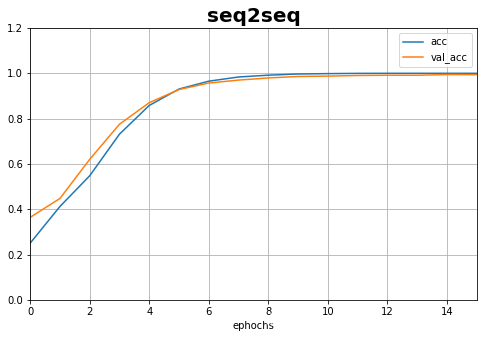
plot_learning_curves(history,'acc',15,0,1.2,title='seq2seq')
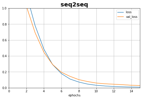
plot_learning_curves(history,'loss',15,0,1,title='seq2seq')

在这里插入图片描述

def define_models(n_input=51, n_output=51, n_units=128): #
    # encoder:
    encoder_inputs = tf.keras.Input(shape = X1.shape[1:])
    encoder = LSTM(n_units, return_state=True,return_sequences=True)
    encoder_ = LSTM(n_units, return_state=True)
    enc_outputs, enc_state_h_, enc_state_c_ = encoder(encoder_inputs)
    enc_outputs_, enc_state_h, enc_state_c = encoder(encoder_inputs)
    #decoder
    dec_states_inputs = [enc_state_h, enc_state_c]
    decoder_inputs = tf.keras.Input(shape = X2.shape[1:])
    decoder_lstm = LSTM(n_units, return_sequences=True, return_state=True)
    dec_outputs,dec_state_h,dec_state_c = decoder_lstm(decoder_inputs,initial_state=dec_states_inputs)
    attention_output = tf.keras.layers.Attention()([dec_outputs,enc_outputs])
    dense_output_ = Dense(n_output, activation='softmax', name="dense")
    dense_outputs = dense_output_(attention_output)
    
    model = Model([encoder_inputs, decoder_inputs], dense_outputs)
    
    # 新序列预测时需要的encoder
    encoder_model = Model(encoder_inputs, dec_states_inputs)
    
    # 新序列预测时需要的decoder
    decoder_state_input_h = Input(shape=(n_units,))
    decoder_state_input_c = Input(shape=(n_units,))
    decoder_states_inputs = [decoder_state_input_h, decoder_state_input_c]
    decoder_outputs, state_h, state_c = decoder_lstm(decoder_inputs, initial_state=decoder_states_inputs)
    decoder_states = [state_h, state_c]
    decoder_outputs = dense_output_(decoder_outputs)
    decoder_model = Model([decoder_inputs] + decoder_states_inputs, [decoder_outputs] + decoder_states)
    
    return model, encoder_model, decoder_model

# one_hot解码
def one_hot_decode(encoded_seq):
	return [argmax(vector) for vector in encoded_seq]
 
# 参数设置
n_features = 50 + 1
n_steps_in = 6
n_steps_out = 3
# 定义模型
train, infenc, infdec = define_models(n_features, n_features, 128)
train.compile(optimizer='adam', loss='categorical_crossentropy', metrics=['acc'])
# 生成训练数据
X1, X2, y = get_dataset(n_steps_in, n_steps_out, n_features, 10000)
print(X1.shape,X2.shape,y.shape)

(10000, 6, 51) (10000, 3, 51) (10000, 3, 51)

history_1 = train.fit([X1, X2], y, epochs=20,validation_split=0.2)

Train on 8000 samples, validate on 2000 samples
Epoch 1/20
8000/8000 [==============================] - 8s 969us/sample - loss: 2.5673 - acc: 0.2918 - val_loss: 1.7339 - val_acc: 0.3510
Epoch 2/20
8000/8000 [==============================] - 2s 236us/sample - loss: 1.5926 - acc: 0.3520 - val_loss: 1.5530 - val_acc: 0.3570
Epoch 3/20
8000/8000 [==============================] - 2s 236us/sample - loss: 1.4423 - acc: 0.3657 - val_loss: 1.4172 - val_acc: 0.3813
Epoch 4/20
8000/8000 [==============================] - 2s 249us/sample - loss: 1.3057 - acc: 0.4116 - val_loss: 1.2525 - val_acc: 0.4455
Epoch 5/20
8000/8000 [==============================] - 2s 229us/sample - loss: 1.0923 - acc: 0.5035 - val_loss: 1.0337 - val_acc: 0.5330
Epoch 6/20
8000/8000 [==============================] - 2s 230us/sample - loss: 0.8598 - acc: 0.6411 - val_loss: 0.8116 - val_acc: 0.7083
Epoch 7/20
8000/8000 [==============================] - 2s 242us/sample - loss: 0.6095 - acc: 0.8219 - val_loss: 0.5731 - val_acc: 0.8387
Epoch 8/20
8000/8000 [==============================] - 2s 242us/sample - loss: 0.4130 - acc: 0.9014 - val_loss: 0.4412 - val_acc: 0.8745
Epoch 9/20
8000/8000 [==============================] - 2s 221us/sample - loss: 0.2984 - acc: 0.9341 - val_loss: 0.3632 - val_acc: 0.8975
Epoch 10/20
8000/8000 [==============================] - 2s 225us/sample - loss: 0.2196 - acc: 0.9573 - val_loss: 0.2985 - val_acc: 0.9168
Epoch 11/20
8000/8000 [==============================] - 2s 226us/sample - loss: 0.1659 - acc: 0.9717 - val_loss: 0.2556 - val_acc: 0.9310
Epoch 12/20
8000/8000 [==============================] - 2s 235us/sample - loss: 0.1274 - acc: 0.9822 - val_loss: 0.2292 - val_acc: 0.9347
Epoch 13/20
8000/8000 [==============================] - 2s 232us/sample - loss: 0.0996 - acc: 0.9879 - val_loss: 0.2066 - val_acc: 0.9397
Epoch 14/20
8000/8000 [==============================] - 2s 228us/sample - loss: 0.0781 - acc: 0.9925 - val_loss: 0.1893 - val_acc: 0.9427
Epoch 15/20
8000/8000 [==============================] - 2s 243us/sample - loss: 0.0619 - acc: 0.9952 - val_loss: 0.1712 - val_acc: 0.9458
Epoch 16/20
8000/8000 [==============================] - 2s 235us/sample - loss: 0.0493 - acc: 0.9968 - val_loss: 0.1641 - val_acc: 0.9495
Epoch 17/20
8000/8000 [==============================] - 2s 224us/sample - loss: 0.0405 - acc: 0.9978 - val_loss: 0.1494 - val_acc: 0.9545
Epoch 18/20
8000/8000 [==============================] - 2s 226us/sample - loss: 0.0328 - acc: 0.9986 - val_loss: 0.1427 - val_acc: 0.9532
Epoch 19/20
8000/8000 [==============================] - 2s 233us/sample - loss: 0.0274 - acc: 0.9990 - val_loss: 0.1403 - val_acc: 0.9563
Epoch 20/20
8000/8000 [==============================] - 2s 223us/sample - loss: 0.0234 - acc: 0.9990 - val_loss: 0.1291 - val_acc: 0.9582

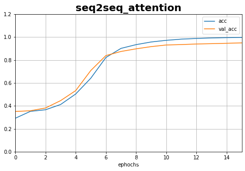
plot_learning_curves(history_1,'acc',15,0,1.2,title='seq2seq_attention')
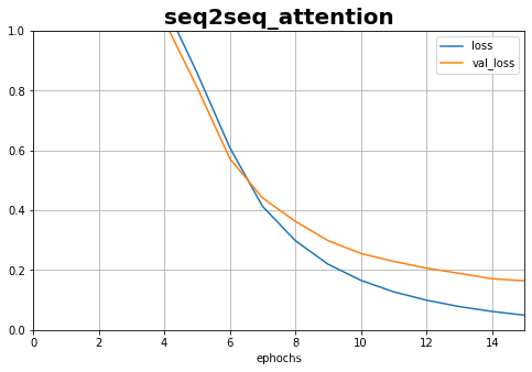
plot_learning_curves(history_1,'loss',15,0,1,title='seq2seq_attention')

在这里插入图片描述

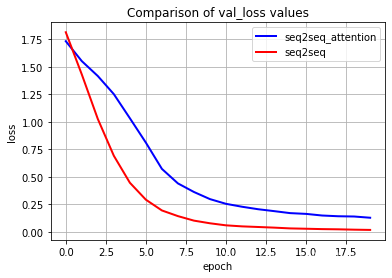
plt.plot(history_1.epoch,history_1.history.get('val_loss'),
         label='seq2seq_attention',color='blue',linewidth='2')
plt.plot(history.epoch,history.history.get('val_loss'),
         label='seq2seq',color='red',linewidth='2')
plt.xlabel('epoch')
plt.ylabel('loss')
plt.title("Comparison of val_loss values")
plt.grid(True)
plt.legend(loc='best')
plt.show()

[外链图片转存失败,源站可能有防盗链机制,建议将图片保存下来直接上传(img-qc8Obs4y-1593876766964)(output_13_0.png)]

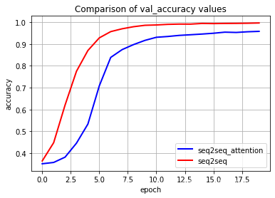
plt.plot(history_1.epoch,history_1.history.get('val_acc'),
         label='seq2seq_attention',color='blue',linewidth='2')
plt.plot(history.epoch,history.history.get('val_acc'),
         label='seq2seq',color='red',linewidth='2')
plt.xlabel('epoch')
plt.ylabel('accuracy')
plt.title("Comparison of val_accuracy values")
plt.grid(True)
plt.legend(loc='best')
plt.show()