python第12周作业——Matplotlib

Exercise 11.1: Plotting a function

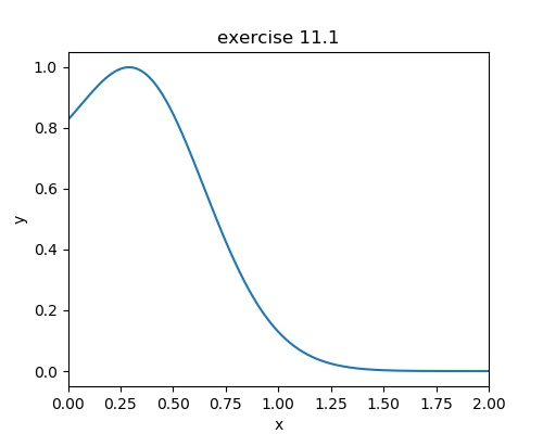
Plot the function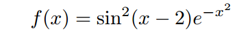 
 
over the interval [0,2]. Add proper axis labels, a title, etc.

代码

import numpy as np
import matplotlib.pyplot as plt
import seaborn as sns

f,ax = plt.subplots(1,1,figsize = (5,4))

x = np.linspace(0,2,1000)
y = np.power(np.sin((x-2)*np.exp((-x*x))),2)
ax.plot(x,y)
ax.set_xlim((0,2))
ax.set_xlabel('x')
ax.set_ylabel('y')
ax.set_title('exercise 11.1')

plt.savefig('exercise 11.1.pdf')

生成图像

Exercise 11.2: Data

Create a data matrix X with 20 observations of 10 variables. Generate a vector b with parameters Then generate the response vector y = Xb+z where z is a vector with standard normally distributed variables. 
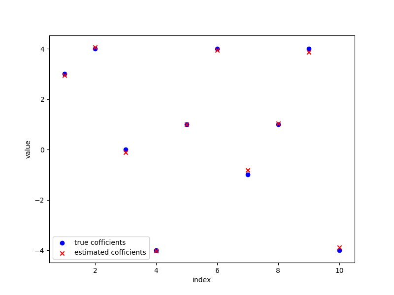
Now (by only using y and X), find an estimator for b, by solving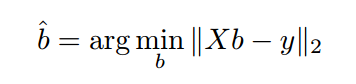 
 
Plot the true parameters b and estimated parameters ^b. See Figure 1 for an example plot. 

代码

import numpy as np
import matplotlib.pyplot as plt
import seaborn as sns
from scipy.optimize import leastsq

#11.2
X = np.random.randint(0,10,(20,10))
b = np.random.randint(-5,5,(1,10))
bt = b.T
z = np.random.randn(20,1)
y = np.dot(X,bt)+z
b_ = np.linalg.lstsq(X, y, rcond=None)[0]
b_t = b_.T

plt.figure(figsize=(8,6))
x = list(range(1,11))
true_b = plt.scatter(x, b, c='b', marker='o', label='true cofficients')
estimated_b = plt.scatter(x, b_t, c='r', marker='x', label='estimated cofficients')
plt.legend()
plt.xlabel('index')
plt.ylabel('value')
plt.savefig('11.2.pdf')

生成图像

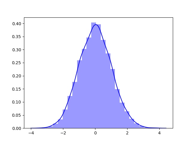
Exercise 11.3: Histogram and density estimation

Generate a vector z of 10000 observations from your favorite exotic distribution. Then make a plot that shows a histogram of z (with 25 bins), along with an estimate for the density, using a Gaussian kernel density estimator (see scipy.stats). See Figure 2 for an example plot.

代码

import numpy as np
import matplotlib.pyplot as plt
import scipy.stats as ss
import seaborn as sns

z = np.random.randn(10000)
sns.distplot(z, bins=25, kde=True,color='b')
plt.savefig('11.3.jpg')

生成图像