


0.1.1. 读取图像形式的MNIST #划分为train/test #对数据进行归一化,即0-1之间,数据要变成float类型 #把数据顺序打乱
'''
导入必须的库
'''
import os
from PIL import Image
import numpy as np
import matplotlib.pyplot as plt
from numpy.ma.extras import unique
'''
根据名称整出来训练集、测试集和对应的标签
'''
def load_images_and_split(folder):
train_images = []
test_images = []
test_labels = []
train_labels = []
for filename in os.listdir(folder):
if filename.endswith('.jpg'):
img_path = os.path.join(folder, filename)
try:
img = Image.open(img_path)
img_array = np.array(img)
label = filename[-5]
if 'test' in filename:
test_images.append(img_array)
try:
# 尝试将标签转换为整数
test_labels.append(int(label))
except ValueError:
print(f"Invalid label in {filename}: {label}. Skipping this image.")
elif 'training' in filename:
train_images.append(img_array)
try:
train_labels.append(int(label))
except ValueError:
print(f"Invalid label in {filename}: {label}. Skipping this image.")
except Exception as e:
print(f"Error loading {img_path}: {e}")
train_images = np.array(train_images)
test_images = np.array(test_images)
train_labels = np.array(train_labels)
test_labels = np.array(test_labels)
return train_images, train_labels, test_images, test_labels
'''
数据预处理,展平和归一化部分在这里
'''
def preprocess_data(train_images, test_images):
# 展平图片数据
train_images_flat = train_images.reshape(train_images.shape[0], -1)
test_images_flat = test_images.reshape(test_images.shape[0], -1)
# 归一化处理
#注意这次必须要进行归一化,否则在后续前向传播的过程中exp会超出精度
train_images_normalized = train_images_flat / 255.0
test_images_normalized = test_images_flat / 255.0
return train_images_normalized, test_images_normalized
'''
onehot编码方便交叉熵损失计算
'''
def one_hot_encode(labels, num_classes):
one_hot = np.zeros((labels.shape[0], num_classes))
one_hot[np.arange(labels.shape[0]), labels] = 1
return one_hot
'''
检查路径和读取
'''
# image_folder = 'mnist_jpg/mnist_jpg'
image_folder = "E:/Strudy/Data/nearestk/mnist_jpg/mnist_jpg"
train_images, test_images,train_labels,test_labels = load_images_and_split(image_folder)
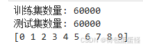
print(f"训练集数量: {len(train_images)}")
print(f"测试集数量: {len(test_images)}")
print(unique(test_labels))
'''
定义评估函数
'''
def two_evaluate_model(test_images, test_labels, weights1, bias1,weights2,bias2,x_row):
    #隐藏
    #本次作业要求使用的是sigmoid激活函数
    #第一层
    hidden_layer=1 / (1 + np.exp(-np.dot(test_images, weights1) + bias1))
    #第二层,注意这里第二层的输出不需要使用任何激活函数
    logits = np.dot(hidden_layer, weights2) + bias2
    y_pred = logits
    predicted_labels = np.argmax(y_pred, axis=1)
    accuracy = np.mean(predicted_labels == test_labels)
    # print(f'Accuracy on the test set: {accuracy * 100}%')

    return accuracy
0.1.2. 参考PPT定义并训练一个两层的神经网络, #定义网络 #损失函数和PPT一致 #中间层激活函数sigmoid
'''
绘图
'''
def drawing(x,y,title):
plt.plot(x,y)
plt.title(title)
plt.show()
'''
SGD
'''
def SGD(test_images_normalized, test_labels, train_images, train_labels, num_classes, num_trials=100, batch_size=100):
#注意,这里输入的x矩阵(也就是图像)和上次课作业不同,本次使用的小批量梯度下降,也就是随机选取batch_size个图像进行梯度的迭代。X是[batch_size,input_size],最终的y_pred输出的维度是[batch_size,10],可以使用print(batch_images.shape)检验一下
input_size = train_images.shape[1]
x_row = [] #这个三个参数纯粹为了画图
y_loss_row = []
y_rate_row = []
# 初始化第一层
weights1 = np.random.randn(input_size, num_classes)
bias1 = np.zeros((1, num_classes))
# 初始化第二层
weights2 = np.random.randn(num_classes, num_classes)
bias2 = np.zeros((1, num_classes))
num_samples = train_images.shape[0]
for trial in range(num_trials):
# 随机打乱样本顺序
permutation = np.random.permutation(num_samples)
shuffled_images = train_images[permutation]
shuffled_labels = train_labels[permutation]
for i in range(0, num_samples, batch_size):
# 取出一个小批量样本
batch_images = shuffled_images[i:i + batch_size]
batch_labels = shuffled_labels[i:i + batch_size]
# 前向传播
# 第一层,使用的是sigmoid函数
hidden_layer = 1 / (1 + np.exp(-np.dot(batch_images, weights1) + bias1))
#第二层,没有激活函数哦
y_pred = np.dot(hidden_layer, weights2) + bias2
# 计算损失,老师课上要求使用的L2损失
y_true = one_hot_encode(batch_labels, num_classes)
loss = np.square((y_pred - y_true)**2).sum()
# 更新参数,也就是上游梯度*当前梯度
grad_y_pred = 2 * (y_pred - y_true)
grad_w2 = hidden_layer.T.dot(grad_y_pred) #对于这行代码,grad_y_gred是上游梯度,乘上中间层输出的转置
grad_b2 = np.sum(grad_y_pred, axis=0, keepdims=True)
#和老师的ppt上内容不同,我用的是y=wx+b,也就是偏置和权重矩阵是分开来的。
grad_h = grad_y_pred.dot(weights2.T)
grad_w1 = batch_images.T.dot(grad_h * hidden_layer * (1 - hidden_layer))#这里用到了sigmoid的求导公式,sigmoid的导数可以用自己表示自己
grad_b1 = np.sum(grad_h * hidden_layer * (1 - hidden_layer), axis=0, keepdims=True)
更新参数,跟着负梯度迭代
weights1 -= 1e-4 * grad_w1
weights2 -= 1e-4 * grad_w2
bias1 -= 1e-4 * grad_b1
bias2 -= 1e-4 * grad_b2
x_row.append(trial)
# 计算当前批次的平均损失
y_loss_row.append(loss)
acc = two_evaluate_model(test_images_normalized, test_labels, weights1, bias1, weights2, bias2,x_row)
y_rate_row.append(acc)
print(f'Trial {trial + 1}, Loss: {loss}')
drawing(x_row, y_loss_row, 'Loss')
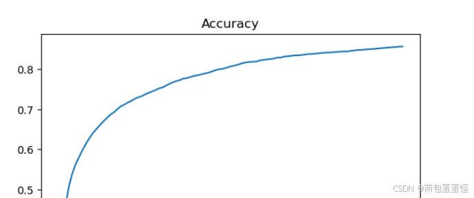
drawing(x_row, y_rate_row, 'Accuracy')
主函数如下调用
image_folder = "E:/Strudy/Data/nearestk/mnist_jpg/mnist_jpg"
train_images, train_labels, test_images, test_labels = load_images_and_split(image_folder)
train_images_normalized, test_images_normalized = preprocess_data(train_images, test_images)
num_classes = len(np.unique(train_labels))
SGD(test_images_normalized, test_labels,train_images_normalized, train_labels, num_classes)
损失图像: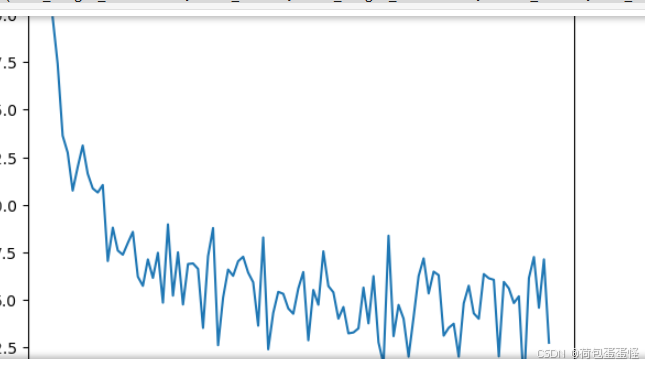
精确度图像:
老师还要求更改epoch和batch_size进行实验,自行修改超参数就可以。
我自己的实验结果是epoch=100和batch_size=100时候的效果最佳。
实验结果分析 1、归一化的重要性:由于本次实验对象维度很大,所以不进行归一化会报错超出float的精度 2、本次实验使用SGD的方法。当batch_size选取为100,进行100次迭代发现实验结果良好,最终准确率是一个平滑的上升曲线,达到了85.7%的精度。 3、扩大batch_size实验发现实验效果很差,并且波动很大。初步猜测是因为迭代次数过少,没有办法学到样本的重要特征。所以在batch_size=1000的基础上扩大epoch=1000,发现实验效果仍然不理想。个人初步认为是样本选取数量变多,但是学习步长太短,更新迭代速率太慢,并且可能陷入了局部最优解。个人在自己电脑跑了一下,发现调整学习率会让准确率提升很多。


 被折叠的 条评论
为什么被折叠?
被折叠的 条评论
为什么被折叠?
 到【灌水乐园】发言


