kaggle泰坦尼克号处理流程

前言

本文探索性数据分析和特征工程部分大量参考了kaggle上的一篇教程，地址：https://www.kaggle.com/ash316/eda-to-prediction-dietanic
这篇文章的内容我花了几天的时间整理出来的，包含了kaggle上竞赛的基本过程，主要内容有探索性数据分析、特征工程、建模、调参

导库并加载数据

import warnings

warnings.filterwarnings('ignore')

import numpy as np
import pandas as pd
import matplotlib.pyplot as plt
import seaborn as sns

train = pd.read_csv('train.csv')
test = pd.read_csv('test.csv')

数据总览

print(train.shape)
train.head()

(891, 12)

	PassengerId	Survived	Pclass	Name	Sex	Age	SibSp	Parch	Ticket	Fare	Cabin	Embarked
0	1	0	3	Braund, Mr. Owen Harris	male	22.0	1	0	A/5 21171	7.2500	NaN	S
1	2	1	1	Cumings, Mrs. John Bradley (Florence Briggs Th...	female	38.0	1	0	PC 17599	71.2833	C85	C
2	3	1	3	Heikkinen, Miss. Laina	female	26.0	0	0	STON/O2. 3101282	7.9250	NaN	S
3	4	1	1	Futrelle, Mrs. Jacques Heath (Lily May Peel)	female	35.0	1	0	113803	53.1000	C123	S
4	5	0	3	Allen, Mr. William Henry	male	35.0	0	0	373450	8.0500	NaN	S

train.tail()

	PassengerId	Survived	Pclass	Name	Sex	Age	SibSp	Parch	Ticket	Fare	Cabin	Embarked
886	887	0	2	Montvila, Rev. Juozas	male	27.0	0	0	211536	13.00	NaN	S
887	888	1	1	Graham, Miss. Margaret Edith	female	19.0	0	0	112053	30.00	B42	S
888	889	0	3	Johnston, Miss. Catherine Helen "Carrie"	female	NaN	1	2	W./C. 6607	23.45	NaN	S
889	890	1	1	Behr, Mr. Karl Howell	male	26.0	0	0	111369	30.00	C148	C
890	891	0	3	Dooley, Mr. Patrick	male	32.0	0	0	370376	7.75	NaN	Q

print(test.shape)
test.head()

(418, 11)

	PassengerId	Pclass	Name	Sex	Age	SibSp	Parch	Ticket	Fare	Cabin	Embarked
0	892	3	Kelly, Mr. James	male	34.5	0	0	330911	7.8292	NaN	Q
1	893	3	Wilkes, Mrs. James (Ellen Needs)	female	47.0	1	0	363272	7.0000	NaN	S
2	894	2	Myles, Mr. Thomas Francis	male	62.0	0	0	240276	9.6875	NaN	Q
3	895	3	Wirz, Mr. Albert	male	27.0	0	0	315154	8.6625	NaN	S
4	896	3	Hirvonen, Mrs. Alexander (Helga E Lindqvist)	female	22.0	1	1	3101298	12.2875	NaN	S

train.describe() #显示数值型特征的描述信息

	PassengerId	Survived	Pclass	Age	SibSp	Parch	Fare
count	891.000000	891.000000	891.000000	714.000000	891.000000	891.000000	891.000000
mean	446.000000	0.383838	2.308642	29.699118	0.523008	0.381594	32.204208
std	257.353842	0.486592	0.836071	14.526497	1.102743	0.806057	49.693429
min	1.000000	0.000000	1.000000	0.420000	0.000000	0.000000	0.000000
25%	223.500000	0.000000	2.000000	20.125000	0.000000	0.000000	7.910400
50%	446.000000	0.000000	3.000000	28.000000	0.000000	0.000000	14.454200
75%	668.500000	1.000000	3.000000	38.000000	1.000000	0.000000	31.000000
max	891.000000	1.000000	3.000000	80.000000	8.000000	6.000000	512.329200

train.describe(include='O') #显示字符串类型的特征描述

	Name	Sex	Ticket	Cabin	Embarked
count	891	891	891	204	889
unique	891	2	681	147	3
top	Backstrom, Mrs. Karl Alfred (Maria Mathilda Gu...	male	1601	C23 C25 C27	S
freq	1	577	7	4	644

train.info()

<class 'pandas.core.frame.DataFrame'>
RangeIndex: 891 entries, 0 to 890
Data columns (total 12 columns):
PassengerId    891 non-null int64
Survived       891 non-null int64
Pclass         891 non-null int64
Name           891 non-null object
Sex            891 non-null object
Age            714 non-null float64
SibSp          891 non-null int64
Parch          891 non-null int64
Ticket         891 non-null object
Fare           891 non-null float64
Cabin          204 non-null object
Embarked       889 non-null object
dtypes: float64(2), int64(5), object(5)
memory usage: 83.6+ KB

各个特征的含义：

• Survived：1代表被救，0代表遇难
• Pclass：票的等级，1最高，3最低
• sex：性别
• age：年龄
• sibsp：兄弟姐妹配偶等同辈的家人的数量
• parch：父母或儿女的数量
• ticket：票号
• fare：花了多少钱
• cabin：客舱号码
• Embarked：登陆的港口

探索性数据分析

通过下面的两个方法可以查看哪些特征是数值型，哪些是字符串，分类的

train.select_dtypes(include='number').columns

Index(['PassengerId', 'Survived', 'Pclass', 'Age', 'SibSp', 'Parch', 'Fare'], dtype='object')

train.select_dtypes(include=['object']).columns

Index(['Name', 'Sex', 'Ticket', 'Cabin', 'Embarked'], dtype='object')

Survived-目标变量

train.Survived.value_counts(normalize=True)

0    0.616162
1    0.383838
Name: Survived, dtype: float64

train.Survived.value_counts()

0    549
1    342
Name: Survived, dtype: int64

sns.countplot('Survived', data=train)

<matplotlib.axes._subplots.AxesSubplot at 0x1bd52c88>

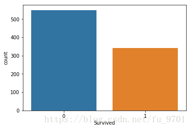
单单只从获救人数来看的话，获救的人数占总人数不多

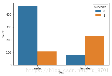
Sex 无序分类变量

train.groupby(['Sex','Survived'])['Survived'].count()

Sex     Survived
female  0            81
        1           233
male    0           468
        1           109
Name: Survived, dtype: int64

pd.crosstab(train.Sex, train.Survived, margins=True) 

Survived	0	1	All
Sex
female	81	233	314
male	468	109	577
All	549	342	891

从这个交叉表可以看出，女性获救概率特别大，可视化会看的更清楚

sns.countplot('Sex', hue='Survived', data=train)

<matplotlib.axes._subplots.AxesSubplot at 0x1bdcb1d0>

Embarked 无序分类变量

train[['Embarked', 'Survived']].groupby('Embarked').sum()

	Survived
Embarked
C	93
Q	30
S	217

pd.crosstab(train.Embarked, train.Survived, margins=True)

Survived	0	1	All
Embarked
C	75	93	168
Q	47	30	77
S	427	217	644
All	549	340	889

sns.countplot('Embarked', hue='Survived', data=train)

<matplotlib.axes._subplots.AxesSubplot at 0x1be2e898>

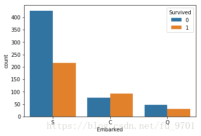
可以看出，虽然从港口S上船的人获救人数最多，但是获救比最高的是从港口C上船的

前面知道，女性获救的概率很大，放到这里再看看：

sns.factorplot('Pclass', 'Survived',hue='Sex', col='Embarked', data=train)

<seaborn.axisgrid.FacetGrid at 0x1bd3de10>

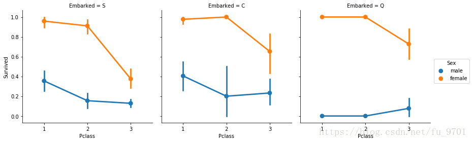
Pclass 有序分类变量

train[['Pclass', 'Survived']].groupby('Pclass').sum(