Coursera深度学习编程作业：Logistic Regression with a Neural Network Mindset

一、Overview of the Problem set

        1. Problem Statement

       给定的数据集中包括：

        - a training set of m_train images labeled as cat (y=1) or non-cat (y=0)
        - a test set of m_test images labeled as cat or non-cat
        - each image is of shape (num_px, num_px, 3) where 3 is for the 3 channels (RGB). Thus, each image is square (height = num_px) and (width = num_px).

        我们需要构造一个简单的图像识别算法，来判断图片是否为cat

        2. load the data

import numpy as np
import copy
import matplotlib.pyplot as plt
import h5py
import scipy
from PIL import Image
from scipy import ndimage
from lr_utils import load_dataset
from public_tests import *

%matplotlib inline
%load_ext autoreload
%autoreload 2

# Loading the data (cat/non-cat)
train_set_x_orig, train_set_y, test_set_x_orig, test_set_y, classes = load_dataset()

        从数据集中直接加载的数据用"_orig"表示。train_set_x_orig为(m_train, num_px, num_px, 3) 的形式，其中每一个line表示一个image的信息；而train_set_y为(m_train,1)的形式。注意m_train, num_px和m_test都没有显式给出，需要通过.shape[]获得：

m_train = train_set_x_orig.shape[0]
m_test = test_set_x_orig.shape[0]
num_px = train_set_x_orig.shape[1]

        3. reshape the image

        为了方便后续的矩阵运算，需要将每个image reshape成(nx, 1)的形式，得到的x用"_flatten"标识

train_set_x_flatten = train_set_x_orig.reshape(m_train, -1).T
test_set_x_flatten = test_set_x_orig.reshape(m_test, -1).T

        4. standardize the dataset

        图像为RBG的表示方法，因此取值范围在[0,255]，通过/255即可标准化，得到最终的training set和test set

train_set_x = train_set_x_flatten / 255.
test_set_x = test_set_x_flatten / 255.

 

二、General Architecture of the learning algorithm

        采用logistic regression作为核心算法，将整个过程视为一个小的神经网络。

        对于每个image  ，依次进行以下计算：

        然后计算总的loss fucntion：

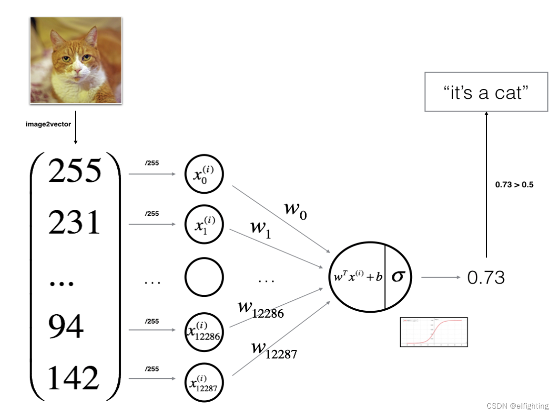
        我们需要进行以下步骤：

        （1）初始化参数w和b

        （2）选择能够最小化J的参数

        （3）利用得到的参数对test set中的数据进行预测

三、Building the parts of our algorithm

        构造神经网络的核心步骤包括：

        （1）确定模型结构（包括input features的个数等）

        （2）初始化参数

        （3）循环：计算current loss(forward propagation)；计算current gradient(backward propagation)；利用gradient descent更新参数

        1. helper function--sigmoid

def sigmoid(z):
    """
    Compute the sigmoid of z

    Arguments:
    z -- A scalar or numpy array of any size.

    Return:
    s -- sigmoid(z)
    """

    #(≈ 1 line of code)
    # s = ...
    # YOUR CODE STARTS HERE
    s = 1/(1+np.exp(-z))
    
    # YOUR CODE ENDS HERE
    
    return s

        2. 初始化参数

        参数w需要被初始化成vector，而不能仅仅设定为w=0；而基于Python自带的broadcasting，b不需要设定为vector，但也要注意的是不要直接b = 0，而是初始化成float形式

# GRADED FUNCTION: initialize_with_zeros

def initialize_with_zeros(dim):
    """
    This function creates a vector of zeros of shape (dim, 1) for w and initializes b to 0.
    
    Argument:
    dim -- size of the w vector we want (or number of parameters in this case)
    
    Returns:
    w -- initialized vector of shape (dim, 1)
    b -- initialized scalar (corresponds to the bias) of type float
    """
    
    # (≈ 2 lines of code)
    # w = ...
    # b = ...
    # YOUR CODE STARTS HERE
    w = np.zeros((dim, 1))
    b = 0.
    
    # YOUR CODE ENDS HERE

    return w, b

        3. Forward and Backward propagation

        将propagation的两个方向同时封装在propagate()函数中，即本函数需要计算出cost function和gradient的大小。

# GRADED FUNCTION: propagate

def propagate(w, b, X, Y):
    """
    Implement the cost function and its gradient for the propagation explained above

    Arguments:
    w -- weights, a numpy array of size (num_px * num_px * 3, 1)
    b -- bias, a scalar
    X -- data of size (num_px * num_px * 3, number of examples)
    Y -- true "label" vector (containing 0 if non-cat, 1 if cat) of size (1, number of examples)

    Return:
    cost -- negative log-likelihood cost for logistic regression
    dw -- gradient of the loss with respect to w, thus same shape as w
    db -- gradient of the loss with respect to b, thus same shape as b
    
    Tips:
    - Write your code step by step for the propagation. np.log(), np.dot()
    """
    
    m = X.shape[1]
    
    # FORWARD PROPAGATION (FROM X TO COST)
    #(≈ 2 lines of code)
    # compute activation
    # A = ...
    # compute cost by using np.dot to perform multiplication. 
    # And don't use loops for the sum.
    # cost = ...                                
    # YOUR CODE STARTS HERE
    A = sigmoid(np.dot(w.T,X)+b) # (1, m)
    cost = -(np.sum(Y*np.log(A)+(1-Y)*np.log(1-A)))/m
    
    # YOUR CODE ENDS HERE

    # BACKWARD PROPAGATION (TO FIND GRAD)
    #(≈ 2 lines of code)
    # dw = ...
    # db = ...
    # YOUR CODE STARTS HERE
    dw = np.dot(X,(A-Y).T)/m
    db = np.sum(A-Y)/m
    
    # YOUR CODE ENDS HERE
    cost = np.squeeze(np.array(cost))

    
    grads = {"dw": dw,
             "db": db}
    
    return grads, cost

        4. Optimzation

        通过gradient descent得到能够使得J最小的参数

# GRADED FUNCTION: optimize

def optimize(w, b, X, Y, num_iterations=100, learning_rate=0.009, print_cost=False):
    """
    This function optimizes w and b by running a gradient descent algorithm
    
    Arguments:
    w -- weights, a numpy array of size (num_px * num_px * 3, 1)
    b -- bias, a scalar
    X -- data of shape (num_px * num_px * 3, number of examples)
    Y -- true "label" vector (containing 0 if non-cat, 1 if cat), of shape (1, number of examples)
    num_iterations -- number of iterations of the optimization loop
    learning_rate -- learning rate of the gradient descent update rule
    print_cost -- True to print the loss every 100 steps
    
    Returns:
    params -- dictionary containing the weights w and bias b
    grads -- dictionary containing the gradients of the weights and bias with respect to the cost function
    costs -- list of all the costs computed during the optimization, this will be used to plot the learning curve.
    
    Tips:
    You basically need to write down two steps and iterate through them:
        1) Calculate the cost and the gradient for the current parameters. Use propagate().
        2) Update the parameters using gradient descent rule for w and b.
    """
    
    w = copy.deepcopy(w)
    b = copy.deepcopy(b)
    
    costs = []
    
    for i in range(num_iterations):
        # (≈ 1 lines of code)
        # Cost and gradient calculation 
        # grads, cost = ...
        # YOUR CODE STARTS HERE
        grads, cost = propagate(w, b, X, Y)
        
        # YOUR CODE ENDS HERE
        
        # Retrieve derivatives from grads
        dw = grads["dw"]
        db = grads["db"]
        
        # update rule (≈ 2 lines of code)
        # w = ...
        # b = ...
        # YOUR CODE STARTS HERE
        w = w - learning_rate*dw
        b = b- learning_rate*db
        
        # YOUR CODE ENDS HERE
        
        # Record the costs
        if i % 100 == 0:
            costs.append(cost)
        
            # Print the cost every 100 training iterations
            if print_cost:
                print ("Cost after iteration %i: %f" %(i, cost))
    
    params = {"w": w,
              "b": b}
    
    grads = {"dw": dw,
             "db": db}
    
    return params, grads, costs

四、预测predict

        首先计算test set中image对应的Yhat，根据Yhat的值（是否大于0.5）判定是否为cat，即Y是否为1。需要特别注意的是，Yhat为(1, m)形式的矩阵，而不是array，因此取值时为[0,i]的格式，Y_prediction也会同样的道理

# GRADED FUNCTION: predict

def predict(w, b, X):
    '''
    Predict whether the label is 0 or 1 using learned logistic regression parameters (w, b)
    
    Arguments:
    w -- weights, a numpy array of size (num_px * num_px * 3, 1)
    b -- bias, a scalar
    X -- data of size (num_px * num_px * 3, number of examples)
    
    Returns:
    Y_prediction -- a numpy array (vector) containing all predictions (0/1) for the examples in X
    '''
    
    m = X.shape[1]
    Y_prediction = np.zeros((1, m))
    w = w.reshape(X.shape[0], 1)
    
    # Compute vector "A" predicting the probabilities of a cat being present in the picture
    #(≈ 1 line of code)
    # A = ...
    # YOUR CODE STARTS HERE
    A = sigmoid(np.dot(w.T,X)+b)
    
    # YOUR CODE ENDS HERE
    
    for i in range(A.shape[1]):
        
        # Convert probabilities A[0,i] to actual predictions p[0,i]
        #(≈ 4 lines of code)
        # if A[0, i] > ____ :
        #     Y_prediction[0,i] = 
        # else:
        #     Y_prediction[0,i] = 
        # YOUR CODE STARTS HERE
        if A[0, i] > 0.5:
            Y_prediction[0,i] = 1
        else:
            Y_prediction[0,i] = 0
        
        # YOUR CODE ENDS HERE
    
    return Y_prediction

五、最终模型

# GRADED FUNCTION: model

def model(X_train, Y_train, X_test, Y_test, num_iterations=2000, learning_rate=0.5, print_cost=False):
    """
    Builds the logistic regression model by calling the function you've implemented previously
    
    Arguments:
    X_train -- training set represented by a numpy array of shape (num_px * num_px * 3, m_train)
    Y_train -- training labels represented by a numpy array (vector) of shape (1, m_train)
    X_test -- test set represented by a numpy array of shape (num_px * num_px * 3, m_test)
    Y_test -- test labels represented by a numpy array (vector) of shape (1, m_test)
    num_iterations -- hyperparameter representing the number of iterations to optimize the parameters
    learning_rate -- hyperparameter representing the learning rate used in the update rule of optimize()
    print_cost -- Set to True to print the cost every 100 iterations
    
    Returns:
    d -- dictionary containing information about the model.
    """
    # (≈ 1 line of code)   
    # initialize parameters with zeros 
    # w, b = ...
    w, b = initialize_with_zeros(X_train.shape[0])
    
    #(≈ 1 line of code)
    # Gradient descent 
    # params, grads, costs = ...
    params, grads, costs = optimize(w, b, X_train, Y_train, num_iterations, learning_rate, print_cost)
    
    # Retrieve parameters w and b from dictionary "params"
    # w = ...
    # b = ...
    w = params["w"] # 注意w是以string的形式作为dict的key，因此必须加上""
    b = params["b"]
    
    # Predict test/train set examples (≈ 2 lines of code)
    # Y_prediction_test = ...
    # Y_prediction_train = ...
    Y_prediction_test = predict(w, b, X_test)
    Y_prediction_train = predict(w, b, X_train)
    

    # Print train/test Errors
    if print_cost:
        print("train accuracy: {} %".format(100 - np.mean(np.abs(Y_prediction_train - Y_train)) * 100))
        print("test accuracy: {} %".format(100 - np.mean(np.abs(Y_prediction_test - Y_test)) * 100))

    
    d = {"costs": costs,
         "Y_prediction_test": Y_prediction_test, 
         "Y_prediction_train" : Y_prediction_train, 
         "w" : w, 
         "b" : b,
         "learning_rate" : learning_rate,
         "num_iterations": num_iterations}
    
    return d