


传统的基于统计的技术
机器自动翻译在2010年之前采用的是基于统计的方法。比如在英译中的应用中,模型为给定英文句子
x
x
x,确定可能性最大的中文句子
y
y
y,即
arg
max
y
P
(
y
∣
x
)
=
arg
max
y
P
(
x
∣
y
)
P
(
y
)
\arg \max_y P(y|x)=\arg\max_y P(x|y)P(y)
argymaxP(y∣x)=argymaxP(x∣y)P(y)
其中
P
(
y
)
P(y)
P(y)即为上文提到的“语言模型”,而
P
(
x
∣
y
)
P(x|y)
P(x∣y)则需要统计大量的中译英的双语句子。在统计
P
(
x
∣
y
)
P(x|y)
P(x∣y),需要考虑到两种语言的“对齐”的特性,比如
- 有些英语单词没有对应的中文词,比如“Let the sun shine in”=》“让 阳光 照 进来”。这里“the”就没有对应的中文翻译词。
- 单个英文单词会对应多个中文词,比如"I am unhappy"=>"我 不 开心“,其中“unhappy”就对应了"不"和“开心”两个中文词。
- 单个中文词会对应多个英文词。比如“Men are not saints"=>"人 非 圣贤“,这里“非”就对应了“are”和“not”两个单词。
- 多个中文词会对应多个英文词。
- 英文词会对应不同位置的中文词。
因此,基于统计的模型会对合适的翻译进行大量的搜索操作,也需要提取不同语言的语法特征,因此实现的复杂度较高。
Seq2Seq模型
自2014年以来,开始出现RNN的技术,可以完全针对不同的语言采用同一类神经网络去训练。只需要给神经网络学习大量的双语例句,就可以让神经网络自动具备翻译的能力。
这里介绍RNN的seq2seq模型。Seq2seq原理是将
P
(
y
∣
x
)
P(y|x)
P(y∣x)分解为
P
(
y
∣
x
)
=
P
(
y
1
∣
x
)
P
(
y
2
∣
y
1
,
x
)
…
P
(
y
T
∣
y
1
,
.
.
.
,
y
T
−
1
,
x
)
P(y|x)=P(y_1|x)P(y_2|y_1,x) \dots P(y_T|y_1,...,y_{T-1},x)
P(y∣x)=P(y1∣x)P(y2∣y1,x)…P(yT∣y1,...,yT−1,x)
其中,
P
(
y
T
∣
y
1
,
.
.
.
,
y
T
−
1
,
x
)
P(y_T|y_1,...,y_{T-1},x)
P(yT∣y1,...,yT−1,x)表示的是给定英文原句
x
x
x和现在已经翻译得到的中文词序列
y
1
,
.
.
.
,
y
T
−
1
y_1,...,y_{T-1}
y1,...,yT−1,判断下一个合适的中文词
y
T
y_T
yT。
下图给出了seq2seq的训练过程。
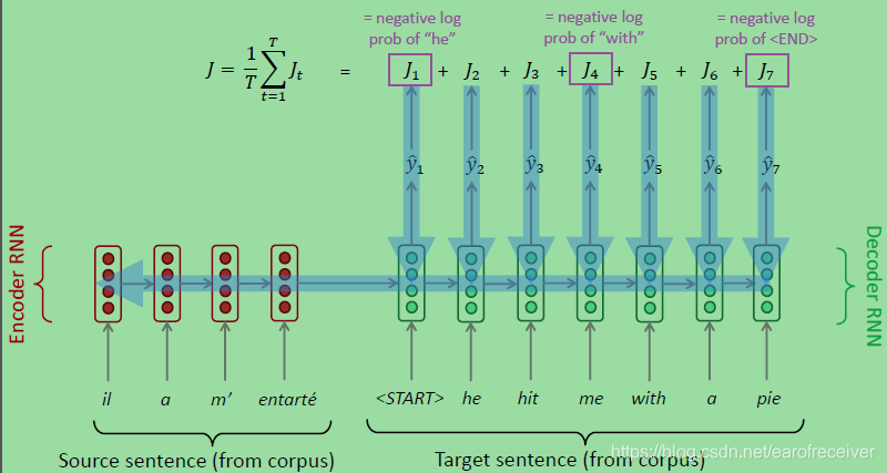
seq2seq包括编码器RNN和解码器RNN两部分。编码器用于对原句进行计算,解码器根据编码器的输出,逐个产生对应的译句的词汇。再将解码器输出的词和语料库的词进行比较,得到损失函数,再通过反向传播计算各节点的梯度。
- 在实现时,编码器的长度是恒定的。因此,需要预先指定或者算出最长的句子的单词数。然后,再对每个原句进行处理,对于没有达到最大长度的句子全部都填上某个特定的字符串,如<pad>
- 解码器的长度则是可变的,根据目标句子的长度不同而不同。
上面仅仅讨论了seq2seq的训练模型。那么如果模型已经训练好,现在在实际进行使用,看会发生什么。
比如输入待翻译的句子,比如在编码器输入序列“I do not want to talk to you”。在第一个解码器经过softmax输出每个中文词出现的概率,这个时候应该取哪个词作为第二个解码器的输入呢?
最为直观的做法是取概率最大的词。但如果恰好解码器输出的“我”的概率为
P
我
=
0.38
P_我=0.38
P我=0.38,而"他"的概率为
P
他
=
0.4
P_他=0.4
P他=0.4。这样就会导致“他”会作为第二个解码器的输入,后面一系列的翻译都会出现问题。
最优的做法是在每一个解码器考虑所有的可能。即在第二个解码器考虑所有可能的
∣
V
∣
|V|
∣V∣个词,再看每个词所有可能的输出,直到最后一级,再求这一组词出现的总概率。很显然,这样做法在第
n
n
n级需要考虑所有
∣
V
∣
n
|V|^n
∣V∣n种可能,显然是不可取的。
还有种次优的做法是beam search,即在每个解码器只考虑概率最大的前
k
k
k个词。假设
k
=
2
k=2
k=2,它的判决过程如下:
上面算法还存在一个问题,就是句子越长,loss越高,因此会导致最高选出来的有可能都是短句子。因此,一般会将计算得到的loss除以句子的长度,即
J
/
T
J/T
J/T。
改进-attention
在seq2seq模型里可以看到,解码器的输入只来自于编码器的最后一级的输出。在上文介绍RNN中可以知道,一个长句子在编码器的最末尾有可能会丢失句首的信息。因此,改进的方法是将每一个编码器的输出,分别和解码器的输出进行“组合”,这样就可以将输入句子中的每一个词的信息都能“带”到每一个解码器中。这样,模型就可以通过训练,自动的发现前面所提到的词汇一对多,多对多,多对一等情况,而不再需要人工的去提取语言的特征了。
这样attention的模型如图所示。
结合上文提到的RNN,模型可以进一步改进:
- 将每一个RNN cell替换为LSTM cell
- 将编码器由单向结构变为双向结构,以充分的利用输入句子正向和反向的信息(如前文所述,针对所谓的“大喘气”的句子,需要反向的信息)。
这样,采用数学表示,完整的结构如下:
给定输入长度为
m
m
m的句子,包括的单词为
x
1
,
.
.
,
x
m
\mathbf{x}_1,..,\mathbf{x}_m
x1,..,xm,其中
x
i
∈
R
e
×
1
\mathbf{x}_i \in \mathbb{R}^{e \times 1}
xi∈Re×1,其中
e
e
e为词向量的长度。句子会被输入到包括双向的LSTM中,前向记为
→
\rightarrow
→,后向记为
←
\leftarrow
←。第
i
i
i个前向LSTM单元会计算
h
i
e
n
c
→
,
c
i
e
n
c
→
=
LSTM
(
x
i
,
h
i
−
1
e
n
c
→
,
c
i
−
1
e
n
c
→
)
\overrightarrow{\mathbf{h}_i^{enc}},\overrightarrow{\mathbf{c}_i^{enc}}=\text{LSTM}(\mathbf{x}_i,\overrightarrow{\mathbf{h}_{i-1}^{enc}},\overrightarrow{\mathbf{c}_{i-1}^{enc}})
hienc,cienc=LSTM(xi,hi−1enc,ci−1enc)
后向单元则计算
h
i
e
n
c
←
,
c
i
e
n
c
←
=
LSTM
(
x
i
,
h
i
+
1
e
n
c
←
,
c
i
+
1
e
n
c
←
)
\overleftarrow{\mathbf{h}_i^{enc}},\overleftarrow{\mathbf{c}_i^{enc}}=\text{LSTM}(\mathbf{x}_i,\overleftarrow{\mathbf{h}_{i+1}^{enc}},\overleftarrow{\mathbf{c}_{i+1}^{enc}})
hienc,cienc=LSTM(xi,hi+1enc,ci+1enc)
这里
h
0
e
n
c
→
,
c
0
e
n
c
→
,
,
h
m
e
n
c
←
,
c
m
e
n
c
←
=
0
\overrightarrow{\mathbf{h}_0^{enc}},\overrightarrow{\mathbf{c}_0^{enc}},,\overleftarrow{\mathbf{h}_{m}^{enc}},\overleftarrow{\mathbf{c}_{m}^{enc}}=\mathbf 0
h0enc,c0enc,,hmenc,cmenc=0.
将第
i
i
i个前向和后向的hidden state
h
i
e
n
c
\mathbf{h}_i^{enc}
hienc和cell state
c
i
e
n
c
\mathbf{c}_i^{enc}
cienc连接起来,即
h
i
e
n
c
=
[
h
i
e
n
c
←
,
h
i
e
n
c
→
]
,
其
中
h
i
e
n
c
∈
R
2
h
×
1
,
,
h
i
e
n
c
←
,
h
i
e
n
c
→
∈
R
h
×
1
\mathbf{h}_i^{enc}=[\overleftarrow{\mathbf{h}_i^{enc}}, \overrightarrow{\mathbf{h}_i^{enc}}],其中\mathbf{h}_i^{enc} \in \mathbb{R}^{2h \times 1}, ,\overleftarrow{\mathbf{h}_i^{enc}}, \overrightarrow{\mathbf{h}_i^{enc}} \in \mathbb{R}^{h \times 1}
hienc=[hienc,hienc],其中hienc∈R2h×1,,hienc,hienc∈Rh×1
以及
c
i
e
n
c
=
[
c
i
e
n
c
←
,
c
i
e
n
c
→
]
,
其
中
c
i
e
n
c
∈
R
2
h
×
1
,
,
c
i
e
n
c
←
,
c
i
e
n
c
→
∈
R
h
×
1
\mathbf{c}_i^{enc}=[\overleftarrow{\mathbf{c}_i^{enc}}, \overrightarrow{\mathbf{c}_i^{enc}}],其中\mathbf{c}_i^{enc} \in \mathbb{R}^{2h \times 1}, ,\overleftarrow{\mathbf{c}_i^{enc}}, \overrightarrow{\mathbf{c}_i^{enc}} \in \mathbb{R}^{h \times 1}
cienc=[cienc,cienc],其中cienc∈R2h×1,,cienc,cienc∈Rh×1
在解码器端,仍然采用单向的RNN(如前文所述,解码器实际对应为“语言模型”,而“语言模型”采用单向RNN是合适的)。第一级解码器的“左侧“输入为编码器的输出的线性变换,即
h
0
d
e
c
=
W
h
[
h
1
e
n
c
←
,
h
m
e
n
c
→
]
,
其
中
h
0
d
e
c
∈
R
h
×
1
,
W
h
∈
R
h
×
2
h
\mathbf{h}_0^{dec}=\mathbf{W}_h[\overleftarrow{\mathbf{h}_1^{enc}}, \overrightarrow{\mathbf{h}_m^{enc}}],其中\mathbf{h}_0^{dec} \in \mathbb{R}^{h \times 1}, \mathbf{W}_h \in \mathbb{R}^{h \times 2h}
h0dec=Wh[h1enc,hmenc],其中h0dec∈Rh×1,Wh∈Rh×2h
以及
c
0
d
e
c
=
W
c
[
c
1
e
n
c
←
,
c
m
e
n
c
→
]
,
其
中
c
0
d
e
c
∈
R
h
×
1
,
W
c
∈
R
h
×
2
h
\mathbf{c}_0^{dec}=\mathbf{W}_c[\overleftarrow{\mathbf{c}_1^{enc}}, \overrightarrow{\mathbf{c}_m^{enc}}],其中\mathbf{c}_0^{dec} \in \mathbb{R}^{h \times 1}, \mathbf{W}_c \in \mathbb{R}^{h \times 2h}
c0dec=Wc[c1enc,cmenc],其中c0dec∈Rh×1,Wc∈Rh×2h
令每一个解码器
t
t
t下方的输入为
y
t
ˉ
\bar{\mathbf {y_t}}
ytˉ(具体表达式在文末给出),则解码器的输入-输出的关系为
h
t
d
e
c
,
c
t
d
e
c
=
LSTM
(
y
t
ˉ
,
h
t
−
1
d
e
c
,
c
t
−
1
d
e
c
)
\mathbf{h}_t^{dec},\mathbf{c}_t^{dec}=\text{LSTM}(\bar{\mathbf {y_t}}, \mathbf{h}_{t-1}^{dec},\mathbf{c}_{t-1}^{dec})
htdec,ctdec=LSTM(ytˉ,ht−1dec,ct−1dec)
其中
h
t
d
e
c
,
c
t
d
e
c
∈
R
h
×
1
\mathbf{h}_t^{dec},\mathbf{c}_t^{dec} \in \mathbb{R}^{h \times 1}
htdec,ctdec∈Rh×1。
现在将解码器的每一个输出和编码器的每一个输出相“连接”,以构造出包含编码器所有信息的数据,这就是前面提到的“attention”,即
e
t
,
i
=
(
h
t
d
e
c
)
T
W
a
t
t
P
r
o
j
h
i
e
n
c
,
其
中
W
a
t
t
P
r
o
j
∈
R
h
×
2
h
e_{t,i}=(\mathbf{h}_t^{dec})^T \mathbf W_{attProj}\mathbf{h}_i^{enc},其中 \mathbf W_{attProj} \in \mathbb{R}^{h \times 2h}
et,i=(htdec)TWattProjhienc,其中WattProj∈Rh×2h
这样对于每一个解码器
t
t
t,其和编码器进行运算后,得到组合信息
e
t
=
(
e
t
,
1
,
.
.
.
,
e
t
,
m
)
T
\mathbf e_t = (e_{t,1},...,e_{t,m})^T
et=(et,1,...,et,m)T,再将其取softmax,即
α
t
=
softmax
(
e
t
)
,
其
中
α
t
∈
R
m
×
1
\mathbf \alpha_t = \text{softmax}(\mathbf e_t),其中\mathbf \alpha_t \in \mathbb{R}^{m \times 1}
αt=softmax(et),其中αt∈Rm×1
这里的
α
t
\mathbf \alpha_t
αt中每一个分量表示输入的句子中的每一个词对当前输出的第
t
t
t个词的影响。然后,对输入的hidden state按照
α
t
\mathbf \alpha_t
αt进行加权平均,就可以得到真正的对当前的输出
t
t
t的词最合适的编码器的hidden state。
a
t
=
∑
i
m
α
t
,
i
h
i
e
n
c
,
其
中
a
t
∈
R
2
h
×
1
\mathbf a_t = \sum_i^m \alpha_{t,i}\mathbf h_i^{enc},其中\mathbf a_t \in \mathbb{R}^{2h \times 1}
at=i∑mαt,ihienc,其中at∈R2h×1
这样,我们将当前解码器
t
t
t输出的hidden state和按照上式计算出来的来自输入的hidden state组合起来,并以此作为对输出词进行判决,即
u
t
=
[
a
t
,
h
t
d
e
c
]
,
u
t
∈
R
3
h
×
1
v
t
=
W
u
u
t
,
v
t
∈
R
h
×
1
,
W
u
∈
R
h
×
3
h
o
t
=
Dropout
(
tanh
v
t
)
,
o
t
∈
R
h
×
1
P
t
=
Softmax
(
W
v
o
c
a
b
o
t
)
,
P
t
∈
R
V
t
a
r
g
e
t
×
1
,
W
v
o
c
a
b
∈
R
V
t
a
r
g
e
t
×
h
\begin{aligned} \mathbf u_t &= [\mathbf a_t, \mathbf h_t^{dec}],\mathbf u_t \in \mathbb{R}^{3h \times 1} \\ \mathbf v_t &= \mathbf W_u \mathbf u_t, \mathbf v_t \in \mathbb{R}^{h \times 1}, \mathbf W_u \in \mathbb{R}^{h \times 3h} \\ \mathbf o_t &= \text{Dropout}(\tanh \mathbf v_t), \mathbf o_t \in \mathbb{R}^{h \times 1} \\ \mathbf P_t &= \text{Softmax}(\mathbf W_{vocab} \mathbf o_t), \mathbf P_t \in \mathbb{R}^{V_{target} \times 1}, \mathbf W_{vocab} \in \mathbb{R}^{V_{target} \times h} \end{aligned}
utvtotPt=[at,htdec],ut∈R3h×1=Wuut,vt∈Rh×1,Wu∈Rh×3h=Dropout(tanhvt),ot∈Rh×1=Softmax(Wvocabot),Pt∈RVtarget×1,Wvocab∈RVtarget×h
其中
∣
V
∣
t
a
r
g
e
t
|V|_{target}
∣V∣target为目标(即汉语)的词库的词个数。对应的第
t
t
t个解码器的loss function为
J
t
=
c
r
o
s
s
e
n
t
r
o
p
y
(
P
t
,
g
t
)
J_t = crossentropy(\mathbf P_t, \mathbf g_t)
Jt=crossentropy(Pt,gt)
其中
g
t
\mathbf g_t
gt为真正输出的1-hot vector。
我们将下一级解码器的"底侧"的输入定义为
y
t
ˉ
=
[
y
t
,
o
t
−
1
]
,
y
t
ˉ
∈
R
(
e
+
h
)
×
1
,
y
t
∈
R
e
×
1
,
o
t
−
1
∈
R
h
×
1
\bar{\mathbf {y_t}} = [\mathbf y_t, \mathbf o_{t-1}], \bar{\mathbf {y_t}} \in \mathbb{R}^{(e+h) \times 1}, \mathbf y_t \in \mathbb{R}^{e \times 1},\mathbf o_{t-1} \in \mathbb{R}^{h \times 1}
ytˉ=[yt,ot−1],ytˉ∈R(e+h)×1,yt∈Re×1,ot−1∈Rh×1
其中
o
0
=
0
\mathbf o_0 = \mathbf 0
o0=0,
y
t
\mathbf y_t
yt为真正输出词的词向量。
这样,就完成了完整的自动翻译深度学习网络的设计。


 被折叠的 条评论
为什么被折叠?
被折叠的 条评论
为什么被折叠?
 到【灌水乐园】发言


